COVID-19: Perturbation dynamics resulting chaos to stable with seasonality transmission

Abstract

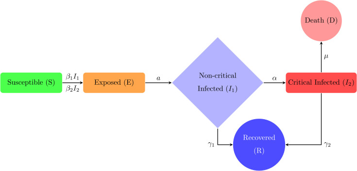
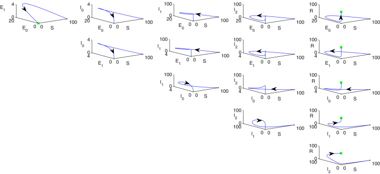
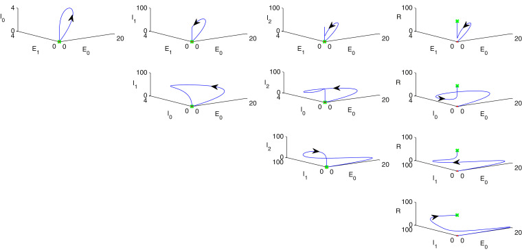
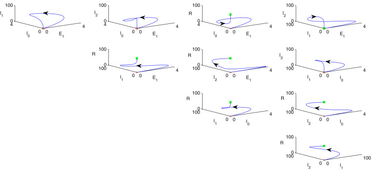
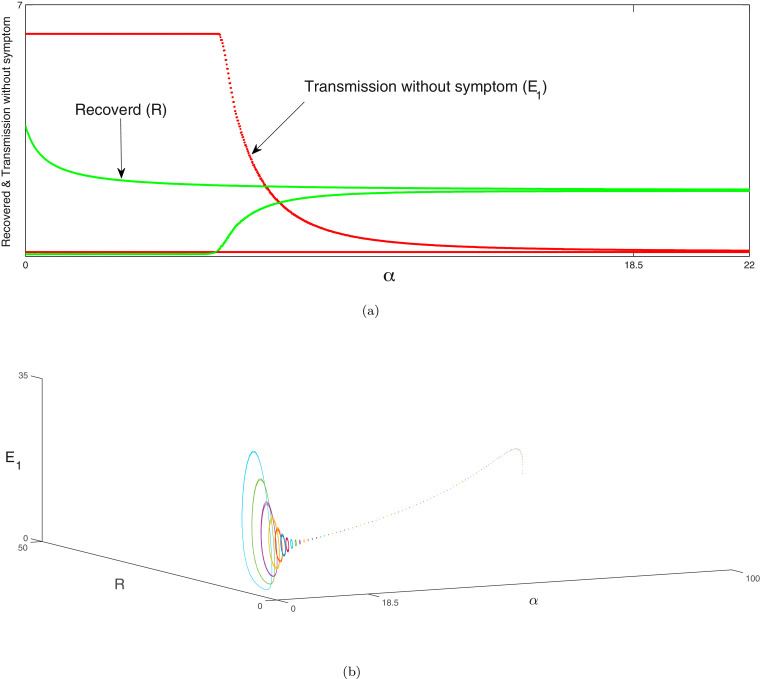
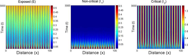
The outbreak of coronavirus is spreading at an unprecedented rate to the human populations and taking several thousands of life all over the globe. In this paper, an extension of the well-known susceptible-exposed-infected-recovered (SEIR) family of compartmental model has been introduced with seasonality transmission of SARS-CoV-2. The stability analysis of the coronavirus depends on changing of its basic reproductive ratio. The progress rate of the virus in critical infected cases and the recovery rate have major roles to control this epidemic. Selecting the appropriate critical parameter from the Turing domain, the stability properties of existing patterns is obtained. The outcomes of theoretical studies, which are illustrated via Hopf bifurcation and Turing instabilities, yield the result of numerical simulations around the critical parameter to forecast on controlling this fatal disease. Globally existing solutions of the model has been studied by introducing Tikhonov regularization. The impact of social distancing, lockdown of the country, self-isolation, home quarantine and the wariness of global public health system have significant influence on the parameters of the model system that can alter the effect of recovery rates, mortality rates and active contaminated cases with the progression of time in the real world.

Keywords: 92B5; 92C60; 92D25; 92D30; Bifurcation analysis; Epidemiology; Mathematical modeling; SARS-CoV-2; Spatial patterns; Stability analysis.

Fig. 1

Extended SEIR model formulation.

Fig. 2

(a) Time series diagram of the model system (1) with the time period of six months. Parameter values of system (1): ${\beta }_1=0.6,{\beta }_2=0.002,a=0.056,\alpha =0.085,{\gamma }_1=0.0025,{\gamma }_2=0.1,\mu =0.02$. (b) Time series diagram of the model system (2) with the time period of six months. Parameter values of system (2): ${\beta }_e=0.045,{\beta }_0=0.025,{\beta }_1=0.025,{\beta }_2=0.025,a_0=1,a_1=5,p=0.07,{\gamma }_0=0.25,{\gamma }_1=0.025,{\gamma }_2=0.015,\alpha =0.1,\mu =0.0125$.

Fig. 3

(i) Simulation of the model system (1) with a lockdown period correspond to the effect of before and after the lockdown. (ii) The effect of mortality rate before and after the lockdown. (iii) The effect of recovered rate before and after the lockdown. (iv) Healthcare capacity system reaches its threshold point at $I=0.1$. Parameter values of system (1): ${\beta }_1=0.6,{\beta }_2=0.002,a=0.056,\alpha =0.085,{\gamma }_1=0.0025,{\gamma }_2=0.1,\mu =0.02$. During the lockdown period ${\beta }_1$ and ${\beta }_2$ are decreased to 0.1 and 0.001 respectively whilst other parameters are fixed. When the lockdown period is over, the value of ${\beta }_1$ is increased to 0.4 (more than lockdown period), however ${\beta }_2$ remains unchanged as 0.001 which implies that after the lockdown is lifted people remain keep social distance with the infected populations.

Fig. 4

Phase portrait diagram of stability analysis w.r.t. all combinations of the individuals of the model system (1), where red point indicates as starting point and the green point denotes the final destination. Parameters are given in Section 11.

Fig. 5

Phase portrait diagram of stability analysis w.r.t. all combinations of the individuals of the model system (2), where red point indicates as starting point and the green point denotes the final destination. Parameters are given in Section 11.

Fig. 6

Phase portrait diagram of stability analysis w.r.t. all combinations of the individuals of the model system (2), where red point indicates as starting point and the green point denotes the final destination. Parameters are given in Section 11.

Fig. 7

Phase portrait diagram of stability analysis w.r.t. all combinations of the individuals of the model system (2), where red point indicates as starting point and the green point denotes the final destination. Parameters are given in Section 11.

Fig. 8

(a) Hopf-bifurcation of susceptible $\left(S\right)$ and recovered $\left(R\right)$ individuals of system (1) corresponding to the bifurcating parameter $\alpha$. The Hopf bifurcation occurs at ${\alpha }_0=0.4$ around the endemic equilibrium. We illustrate the unstable focus on the range ${\alpha }_0<0.4$ and asymptotically stable on the range ${\alpha }_0>0.4$. (b) The three-dimensional diagram of Hopf-bifurcation of the system (1) w.r.t. the parameter of bifurcation $\alpha$ which is portrayed in 3D space which is $(\alpha ,R,S)$. In this Figure endemic equilibria be a focus which is unstable on the range $\alpha <0.4$ (which is depictured with various coloured cycles) and also the endemic equilibria be a focus which is stable on the range $\alpha >0.4$ (depictured with the dashed line). A Hopf-bifurcation takes place at $\alpha =0.4={\alpha }_0$. Other parameters are given in Section 11.

Fig. 9

(a), (b) Hopf-bifurcation of exposed $\left(E\right)$ and non-critical $\left(I_1\right)$ individuals of system (1) corresponding to the bifurcating parameter $\alpha$ respectively. The Hopf bifurcation occurs at ${\alpha }_0=0.4$ around the endemic equilibrium. We illustrate the unstable focus on the range ${\alpha }_0<0.4$ and asymptotically stable on the range ${\alpha }_0>0.4$. (c) The three-dimensional diagram of Hopf-bifurcation of the system (1) w.r.t. the parameter of bifurcation $\alpha$ which is portrayed in 3D space which is $(\alpha ,E,I_1)$. In this Figure endemic equilibria be a focus which is unstable on the range $\alpha <0.4$ (which is depictured with various coloured cycles) and also the endemic equilibria be a focus which is stable on the range $\alpha >0.4$ (depictured with the dashed line). A Hopf-bifurcation takes place at $\alpha =0.4={\alpha }_0$. Other parameters are given in Section 11.

Fig. 10

(a), (b) Hopf-bifurcation of non-critical $\left(I_1\right)$ and critical $\left(I_2\right)$ individuals of system (1) corresponding to the bifurcating parameter $\alpha$ respectively. The Hopf bifurcation occurs at ${\alpha }_0=0.4$ around the endemic equilibrium. We illustrate the unstable focus on the range ${\alpha }_0<0.4$ and asymptotically stable on the range ${\alpha }_0>0.4$. (c) The three-dimensional diagram of Hopf-bifurcation of the system (1) w.r.t. the parameter of bifurcation $\alpha$ which is portrayed in 3D space which is $(\alpha ,I_2,I_1)$. In this Figure endemic equilibria be a focus which is unstable on the range $\alpha <0.4$ (which is depictured with various coloured cycles) and also the endemic equilibria be a focus which is stable on the range $\alpha >0.4$ (depictured with the dashed line). A Hopf-bifurcation takes place at $\alpha =0.4={\alpha }_0$. Other parameters are given in Section 11.

Fig. 11

(a), (b), (c) Hopf-bifurcation of susceptible $\left(S\right),$ no symptom or transmission $\left(E_0\right)$ and asymptomatic infected $\left(I_0\right)$ individuals of system (2) corresponding to the bifurcating parameter $\alpha$ respectively. The Hopf bifurcation occurs at ${\alpha }_0=18.5$ around the endemic equilibrium. We illustrate the unstable focus on the range ${\alpha }_0<18.5$ and asymptotically stable on the range ${\alpha }_0>18.5$. Other parameters are given in Section 11.

Fig. 12

(a), (b) Hopf-bifurcation of non-critical $\left(I_1\right)$ and critical $\left(I_2\right)$ individuals of system (2) corresponding to the bifurcating parameter $\alpha$ respectively. The Hopf bifurcation occurs at ${\alpha }_0=18.5$ around the endemic equilibrium. We illustrate the unstable focus on the range ${\alpha }_0<18.5$ and asymptotically stable on the range ${\alpha }_0>18.5$. (c) The three-dimensional diagram of Hopf-bifurcation of the system (2) w.r.t. the parameter of bifurcation $\alpha$ which is portrayed in 3D space which is $(\alpha ,I_2,I_1)$. In this Figure endemic equilibria be a focus which is unstable on the range $\alpha <18.5$ (which is depictured with various coloured cycles) and also the endemic equilibria be a focus which is stable on the range $\alpha >18.5$ (depictured with the dashed line). A Hopf-bifurcation takes place at $\alpha =18.5={\alpha }_0$. Other parameters are given in Section 11.

Fig. 13

(a) Hopf-bifurcation of transmission without symptom $\left(E_1\right)$ and recovered $\left(R\right)$ individuals of system (2) corresponding to the bifurcating parameter $\alpha$. The Hopf bifurcation occurs at ${\alpha }_0=18.5$ around the endemic equilibrium. We illustrate the unstable focus on the range ${\alpha }_0<18.5$ and asymptotically stable on the range ${\alpha }_0>18.5$. (c) The three-dimensional diagram of Hopf-bifurcation of the system (2) w.r.t. the parameter of bifurcation $\alpha$ which is portrayed in 3D space which is $(\alpha ,R,E1)$. In this Figure endemic equilibria be a focus which is unstable on the range $\alpha <18.5$ (which is depictured with various coloured cycles) and also the endemic equilibria be a focus which is stable on the range $\alpha >18.5$ (depictured with the dashed line). A Hopf-bifurcation takes place at $\alpha =18.5={\alpha }_0$. Other parameters are given in Section 11.

Fig. 14

Snapshots of spatial Turing pattern formations of 1D diffusive parameter w.r.t. the evolution of time of exposed $\left(E\right),$ non-critical infected $\left(I_1\right)$ and critical infected $\left(I_2\right)$ individuals over xt-domain of the system (27) have been portraited. Time, $t=3,000$ has been considered. Perturbation around the endemic equilibria has been considered by $0.5\times {\sin }^2\left(10x\right)$.

Fig. 15

One-dimensional numerical solutions of population ratio with space series and snapshots of contour pictures of the time evolution of exposed $\left(E\right),$ non-critical infected $\left(I_1\right)$ and critical infected $\left(I_2\right)$ individuals in the $xy$-plane of the diffusive model (18) for different values of diffusion parameters (a) $D_1=D_2=D_3=0.001,$ (b) $D_1=D_2=D_3=0.25$ and (c) $D_1=D_2=D_3=2.5,$ incorporating the effect of diffusion parameters $D_1,$$D_2$ and $D_3$ of the system (18). Here, Blue line describes exposed $\left(E\right)$ population, Red line denotes non-critical $\left(I_1\right)$ individual and Green line indicates for critical $\left(I_2\right)$ population.

References

1. Batabyal A., Jana D. Significance of additional food to mutually interfering predator under herd behavior of prey on the stability of a spatio-temporal system. Communications in Nonlinear Science and Numerical Simulation. 2020;93:105480.
1. Jajarmi A., Baleanu D. On the fractional optimal control problems with a general derivative operator. Asian J Control. 2019:1–10. doi: 10.1002/asjc.2282. - DOI
1. Jajarmi A., Baleanu D. A new iterative method for the numerical solution of high-order non-linear fractional boundary value problems. Frontiers in Physics. 2020;8:220.
1. Kucharski A.J., Russell T.W., Diamond C., Liu Y., Edmunds W.J., Funk S., Eggo R.M. Early dynamics of transmission and control of COVID-19 in wuhan. Lancet Infectious Diseases. 2020 - PMC - PubMed
1. Turing A.M. The chemical basis of mokphogenesis, philos. Trans R Soc Lond. 1952;237:37–72.
LinkOut - more resources