Cumulative dietary risk assessment of chronic acetylcholinesterase inhibition by residues of pesticides

Abstract

A retrospective cumulative risk assessment of dietary exposure to pesticide residues was conducted for chronic inhibition of acetylcholinesterase. The pesticides considered in this assessment were identified and characterised in a previous scientific report on the establishment of cumulative assessment groups of pesticides for their effects on the nervous system. The exposure assessments used monitoring data collected by Member States under their official pesticide monitoring programmes in 2016, 2017 and 2018, and individual food consumption data from 10 populations of consumers from different countries and from different age groups. Exposure estimates were obtained by means of a two-dimensional probabilistic model, which was implemented in SAS ^® software. The characterisation of cumulative risk was supported by an uncertainty analysis based on expert knowledge elicitation. For each of the 10 populations, it is concluded with varying degrees of certainty that cumulative exposure to pesticides contributing to the chronic inhibition of acetylcholinesterase does not exceed the threshold for regulatory consideration established by risk managers.

Keywords: acetylcholinesterase inhibition; cumulative risk assessment; knowledge elicitation; pesticide residues; probabilistic modelling.

Figure 1

General process for calculating chronic cumulative exposure to pesticides

Figure 2

Overview of the approach to characterising overall uncertainty in the CRA

Figure 3

Scale used by the experts when assessing EKE Question 1

Figure 4

CAG‐NCN: Consensus distribution of the experts for the combined impact of the quantified uncertainties affecting toxicology (if resolved) on the MOET at the 99.9th percentile of exposure for the Italian adult population in 2016–2018, expressed as a multiplicative factor f to be applied to the Tier II median estimate shown in Table 14. The probability distribution is shown by the curve, which represents the probability density (relative likelihood) for different values of the multiplicative factor f. Distribution parameters are shown in Table 19

Figure 5

CAG‐NCN: Consensus distribution of the experts for the combined impact of the quantified uncertainties affecting exposure (if resolved) on the MOET at the 99.9th percentile of exposure for the Italian adult population in 2016‐2018, expressed as a multiplicative factor f to be applied to the Tier II median estimate shown in Table 14. Distribution parameters are shown in Table 20. Graph content is explained in Figure 4

Figure 6

CAG‐NCN: ‘Model’ boxplots show the output of the Tier II model for the MOET at the 99.9th percentile of exposure in each consumer population in 2016–2018. ‘Model+experts’ boxplots show the result of combining the output of the Tier II model with the elicited distributions quantifying additional sources of uncertainty related to toxicology and exposure, assuming perfect independence between them. Note that the vertical axis is plotted on a logarithmic scale; the values plotted for ‘model+experts’ are shown numerically in Table 21. A key to the populations and explanation of the boxplots are provided in the footnote below the graph

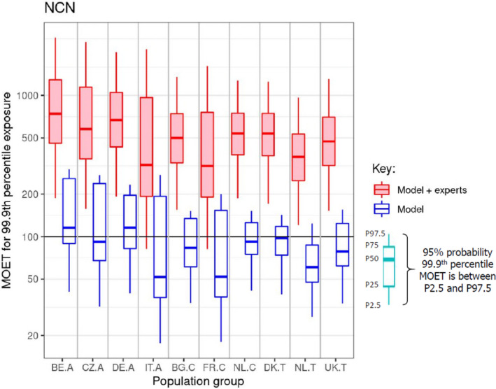
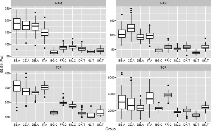
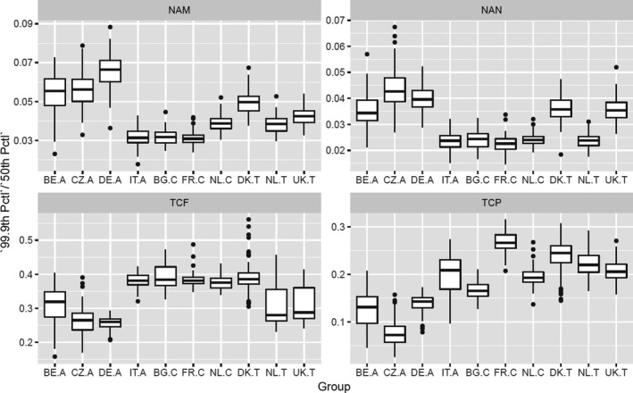
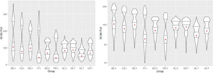
1. Keys: Population groups: BE.A (Belgian adults), CZ.A (Czech Republic adults), DE.A (German adults), IT.A (Italian adults), BG.C (Bulgarian children), FR.C (French children), NL.C (Dutch children), DK.T (Danish toddlers), NL.T (Dutch toddlers), UK.T (United Kingdom toddlers). The lower and upper edges of each boxplot represent the quartiles (P25 and P75) of the uncertainty distribution for each estimate, the horizontal line in the middle of the box represents the median (P50) and the ‘whiskers’ above and below the box show the 95% probability interval (P2.5 and P97.5).

Figure E.1

Density plot for a skewed distribution (lognormal)

Figure E.2

Density plot of the observed 99.9th percentile of 1,000 simulated samples (each with a sample size of 1,000 values)

Figure E.3

Boxplots of 99.9th percentiles from MCRA bootstrap samples for the different consumer groups. NAM, NAN, TCF and TCP refer to CAG‐NAM, CAG‐NAN, CAG‐TCF and CAG‐TCP, respectively

Figure E.4

Boxplots of the ratio of the 99.9th percentile to the 50th percentile from MCRA bootstrap samples for the different consumer groups. NAM, NAN, TCF and TCP refer to CAG‐NAM, CAG‐NAN, CAG‐TCF and CAG‐TCP, respectively

Figure E.5

Violin plots for the confidence intervals of the MOET at the 99.9th percentile of the exposure distributions presented by population (500 bootstraps). The horizontal lines are at quartiles and median, i.e. the ends of the box and the median line in normal boxplots. The width of violin is proportional to density of observation for each value of the MOET at the 99.9th percentile of the exposure distribution. The first version has a linear axis and the second a logarithmic axis. Roughly 3/8 of the samples are in the upper cluster (for all populations where there is clear separation). The nominal run is indicated by a red point and is consistently below the median

Figure G.1

First provisional consensus distribution. Scaled Beta with median of 1.04 and 95% probability interval of 0.69–1.48

Figure G.2

Second provisional consensus distribution. Scaled Beta with median of 1.05 and 95% probability interval of 0.67–1.54

Figure G.3

Third provisional consensus distribution. This is a Log Student‐t distribution truncated at 0.5 and 2. Considering only the part of the distribution which is shown in this figure, the median is 1.05 and 95% probability interval of 0.63–1.69. See Figure G.4 for the non‐truncated version of this distribution

Figure G.4

Comparison of the three provisional consensus distributions. Consensus #1, #2 and #3 correspond to the distributions shown in Figures G.1, G.2 and G.3, respectively. Note that distribution #3 is truncated at the consensus plausible bounds of 0.5 and 2 in Figure G.3, but actually extends beyond those bounds at both ends as can be seen here. The non‐truncated version of consensus distribution #3 has a median of 1.04 and 95% probability interval of 0.56–1.97

Figure G.5

Alternative distributions proposed by experts A, C and D plus the second distribution from the preceding round of consultation and a suggestion from the Facilitator

Figure G.6

Consensus distribution for the multiplicative factor by which the median MOET at the 99.9th percentile of exposure for chronic inhibition of erythrocyte AChE in the Italian adult population at Tier II P99.9 would change if all the identified sources of uncertainty relating to toxicology were resolved. This is a Scaled beta distribution with alpha = 3.15, beta = 4.6 and limits of 0.5 and 2. The red line shows f = 1, i.e. no change in MOET

Figure G.7

Alternative distribution, which was also considered reasonable by the experts, though less preferred than the distribution in Figure G.6 and will be used in sensitivity analysis. This is a Scaled beta distribution with alpha = 3.39 and beta 5.60, beta = 4.6 and limits of 0.5 and 2. The red line shows f = 1, i.e. no change in MOET

Figure H.1

First provisional consensus distribution. Scaled Beta with median of 5.00 and 90% probability interval of 2.81–7.54

Figure H.2

Consensus distribution. Scaled Beta with median of 5.50 and 90% probability interval of 3.15–7.97

References

-
- Abd‐Elhakim YM, El‐Sharkawy NI, Mohammed HH, Ebraheim LLM and Shalaby MA, 2020. Camel milk rescues neurotoxic impairments induced by fenpropathrin via regulating oxidative stress, apoptotic, and inflammatory events in the brain of rats. Food and Chemical Toxicology, 135, 111055 10.1016/j.fct.2019.111055 - DOI - PubMed
- Ahmad I, Shukla S, Kumar A, Singh BK, Patel DK, Pandey HP and Singh C, 2010. Maneb and paraquat‐induced modulation of toxicant responsive genes in the rat liver: comparison with polymorphonuclear leukocytes. Chemico‐Biological Interactions, 188, 566–579. - PubMed
- Ansari RW, Shukla RK, Yadav RS, Seth K, Pant AB, Singh D, Agrawal AK, Islam F and Khanna VJ, 2012. Cholinergic Dysfunctions and Enhanced Oxidative Stress in the Neurobehavioral Toxicity of Lambda‐Cyhalothrin in Developing Rats. Neurotoxicity Research, 22, 292–309. 10.1007/s12640-012-9313-z - DOI - PubMed
- Banerjee BD, Seth V, Bhattacharya A, Pasha ST and Chakraborty AK, 1999. Biochemical effects of some pesticides on lipid peroxidation and free‐radical scavengers. Toxicology Letters, 107, 33–47. - PubMed
LinkOut - more resources
Full Text Sources
Other Literature Sources