The inverse variance-flatness relation in stochastic gradient descent is critical for finding flat minima

Abstract

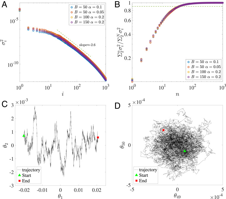
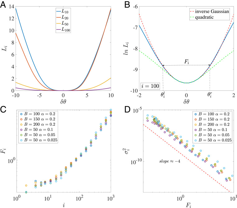
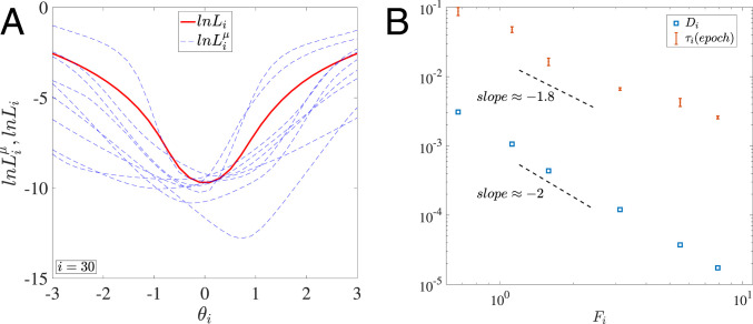
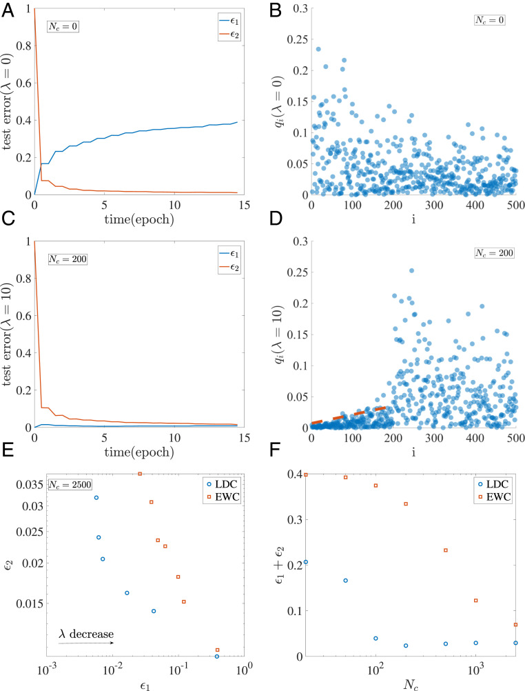
Despite tremendous success of the stochastic gradient descent (SGD) algorithm in deep learning, little is known about how SGD finds generalizable solutions at flat minima of the loss function in high-dimensional weight space. Here, we investigate the connection between SGD learning dynamics and the loss function landscape. A principal component analysis (PCA) shows that SGD dynamics follow a low-dimensional drift-diffusion motion in the weight space. Around a solution found by SGD, the loss function landscape can be characterized by its flatness in each PCA direction. Remarkably, our study reveals a robust inverse relation between the weight variance and the landscape flatness in all PCA directions, which is the opposite to the fluctuation-response relation (aka Einstein relation) in equilibrium statistical physics. To understand the inverse variance-flatness relation, we develop a phenomenological theory of SGD based on statistical properties of the ensemble of minibatch loss functions. We find that both the anisotropic SGD noise strength (temperature) and its correlation time depend inversely on the landscape flatness in each PCA direction. Our results suggest that SGD serves as a landscape-dependent annealing algorithm. The effective temperature decreases with the landscape flatness so the system seeks out (prefers) flat minima over sharp ones. Based on these insights, an algorithm with landscape-dependent constraints is developed to mitigate catastrophic forgetting efficiently when learning multiple tasks sequentially. In general, our work provides a theoretical framework to understand learning dynamics, which may eventually lead to better algorithms for different learning tasks.

Keywords: generalization; loss landscape; machine learning; statistical physics; stochastic gradient descent.

Fig. 1.

The PCA results and the drift–diffusion motion in SGD. (A) The rank-ordered variance ${\sigma }_i^2$ in different principal component (PC) directions $i$. For $i\ge 20$, ${\sigma }_i^2$ decreases with $i$ as a power law $i^{-\gamma }$ with $\gamma \sim 2-3$. (B) The normalized accumulative variance of the top $\left(n-1\right)$ PCs excluding $i=1$. It reaches $\sim 90\%$ at $n=35$ much smaller than the total number of weights $N=\mathrm{2,500}$ between the two hidden layers. (C) The SGD weight trajectory projected onto the $\left({\theta }_1,{\theta }_2\right)$ plane. The persistent drift motion in ${\theta }_1$ and the diffusive random motion in ${\theta }_2$ are clearly shown. (D) The diffusive motion in the $\left({\theta }_i,{\theta }_j\right)$ plane with $j>i\left(\ne \hspace{0.17em}1\right)$ randomly chosen ($i=49$ and $j=50$ shown here). Unless otherwise stated, hyperparameters used are $B=50$, $\alpha =0.1$.

Fig. 2.

The loss function landscape and the inverse variance–flatness relation. (A) The loss function profile $L_i$ along the $i$th PCA direction. (B) The loss landscape (in log-scale). $L_i$ can be fitted better by an inverse Gaussian (the red dashed line) than a quadratic function (the green dashed line). The definition of the flatness $F_i\left(\equiv {\theta }_i^r-{\theta }_i^l\right)$ is also shown (see text for details). (C and D) The flatness $F_i$ for different PCA directions $i$ (C) and the inverse relation between the variance ${\sigma }_i^2$ and the flatness $F_i$ for different choices of minibatch size $B$ and learning rate $\alpha$ (D).

Fig. 3.

Statistical properties of the MLF ensemble. (A) Profiles of the overall loss function $\ln \left(L_i\right)$ (red line) and a set of randomly chosen MLFs $\ln \left(L_i^{\mu }\right)$ (blue dashed lines) in a given PCA direction $i$. (B) The inverse dependence of $D_i$ and ${\tau }_i$ on the flatness $F_i$.

Fig. 4.

The landscape-dependent constraints for avoiding catastrophic forgetting. (A) The test errors for task 1 (${ϵ}_1$) and task 2 (${ϵ}_2$) versus training time for task 2 in the absence of the constraints ($\lambda =0$). (B) The weight displacements $q_i$ in different PCA directions ${\overrightarrow{p}}_{1i}$ from task 1 in the absence of the constraints ($\lambda =0$). C and D are the same as A and B but in the presence of the constraints with $\lambda =10$ and $N_c=200$. The red dashed line in D shows the upper bound $q_i\lesssim 0.008F_{i1}$ for the modes ($i\le N_c$) that are under constraint. (E) The tradeoff between the saturated test errors (${ϵ}_1$ and ${ϵ}_2$) when varying $\lambda$ for LDC (blue circles) and EWC (red squares) algorithms. (F) The overall performance (${ϵ}_1+{ϵ}_2$) versus the number of constrains $N_c$ for LDC (blue circles) and EWC (red squares) algorithms. The two tasks are for classifying two separate digit pairs [$\left(\mathrm{0,1}\right)$ for task 1 and $\left(\mathrm{2,3}\right)$ for task 2] in MNIST.

Fig. 5.

Profiles and dynamics of the anisotropic active temperature. (A) The active temperature profile $T_i\left(\delta \theta ,t\right)$ in the $i$th PCA direction at $t=200$. (B) The minimum active temperature $T_i\left(0\right)$ in different PCA directions $i$. Inset shows the inverse dependence of $T_i$ on the flatness $F_i$. (C) The active temperature profiles $T_i\left(\delta \theta ,t\right)$ at different times for $i=10$. (D) The active temperature $T_i$ for all directions decreases with time in sync with the loss function (red line) dynamics. The shaded region highlights the transition between the fast-learning phase and the exploration phase. Inset shows the correlation between $T_i$ and $L$.

Fig. 6.

The flatness spectrum and the effective dimension ($D_s$) of solution. (A) The flatness spectra (rank-ordered flatness) for networks with different width ($H$). (B) The effective dimension of the solution $D_s$, which is defined as the number of directions whose flatness is below a threshold set to be roughly half of the $L_2$ norm of the weights (the dashed line in A), increases weakly as the number of parameters (weights) $N_p\left(\equiv H^2\right)$ increases. The error bars are obtained by using 10 different solutions obtained by 10 random initializations with the same norm for each network size.

References

-
- LeCun Y., Bengio Y., Hinton G., Deep learning. Nature 521, 436–444 (2015). - PubMed
- Robbins H., Monro S., A stochastic approximation method. Ann. Math. Stat. 22, 400–407 (1951).
- Bottou L. “Large-scale machine learning with stochastic gradient descent” in Proceedings of COMPSTAT’2010, Lechevallier Y., Saporta G., Eds. (Physica-Verlag HD, Heidelberg, Germany, 2010), pp. 177–186.
- Hinton G. E., van Camp D., “Keeping the neural networks simple by minimizing the description length of the weights” in Proceedings of the Sixth Annual Conference on Computational Learning Theory, COLT ‘93, L. Pitt, Ed. (ACM, New York, NY, 1993), pp. 5–13.
- Hochreiter S., Schmidhuber J., Flat minima. Neural Comput. 9, 1–42 (1997). - PubMed
LinkOut - more resources
Full Text Sources
Other Literature Sources