Time Course of Alterations in Adult Spinal Motoneuron Properties in the SOD1(G93A) Mouse Model of ALS

Abstract

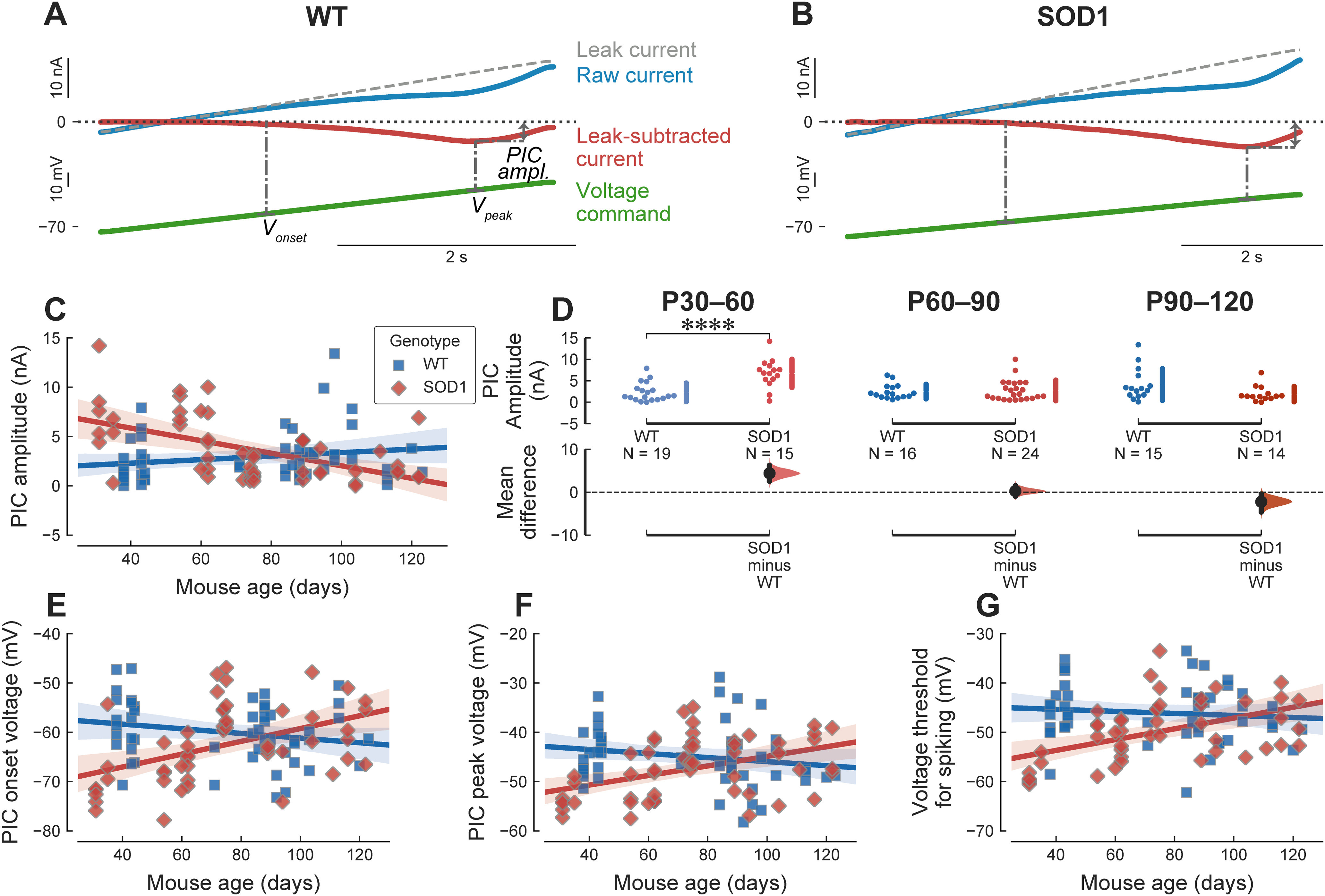
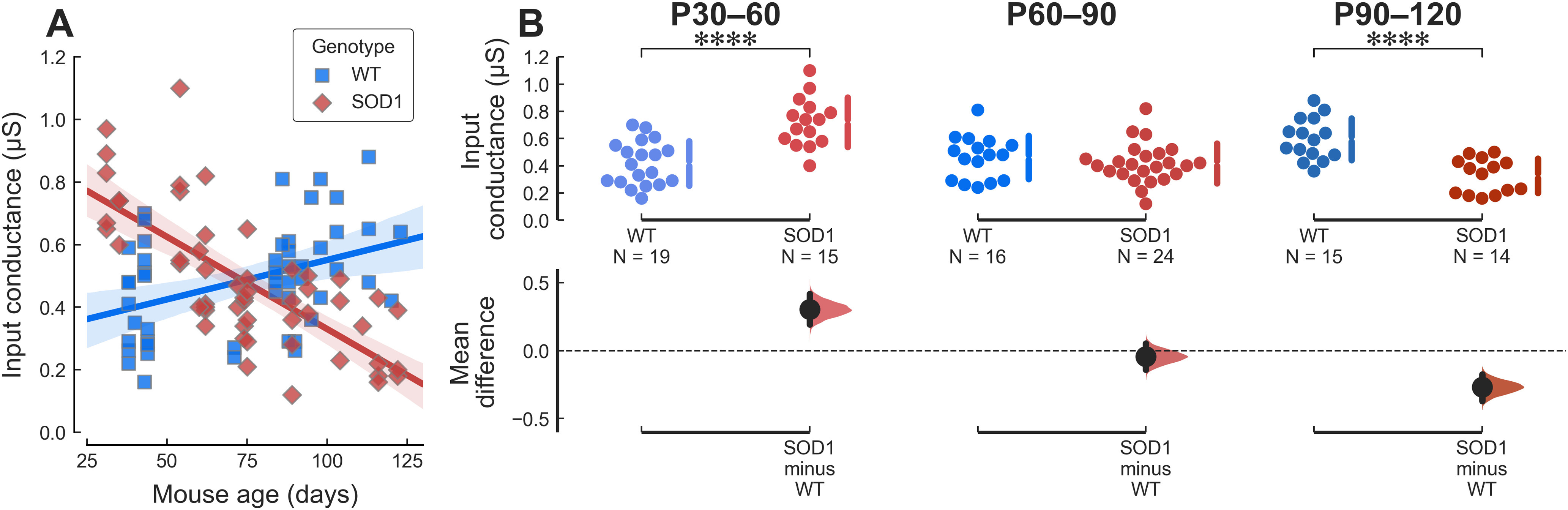
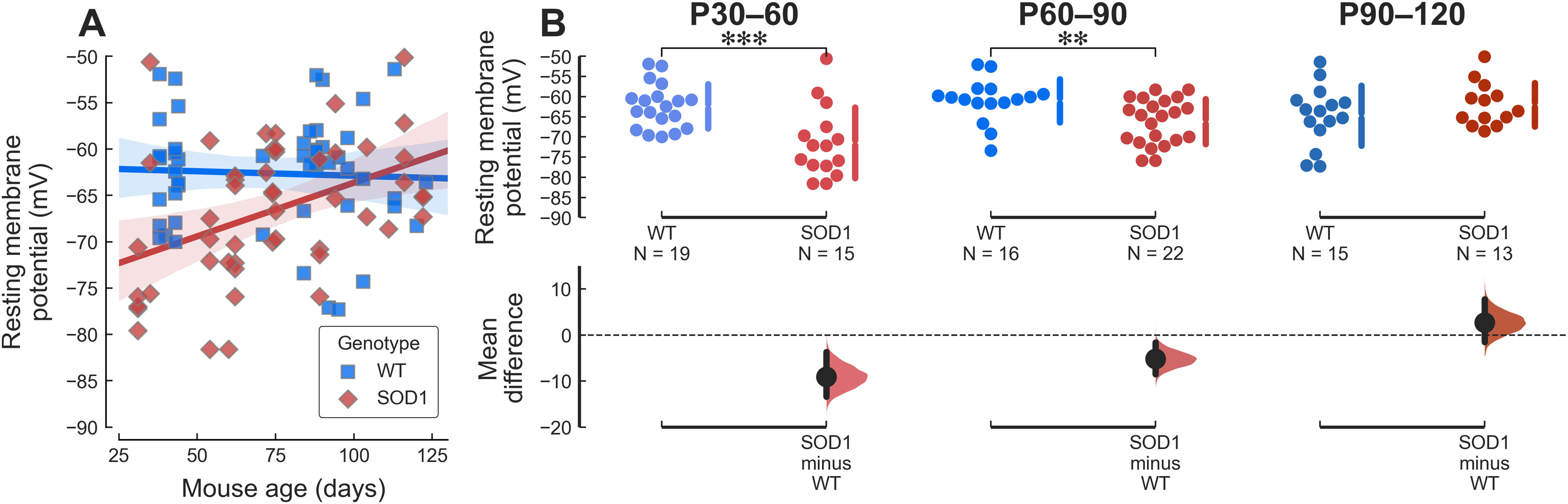
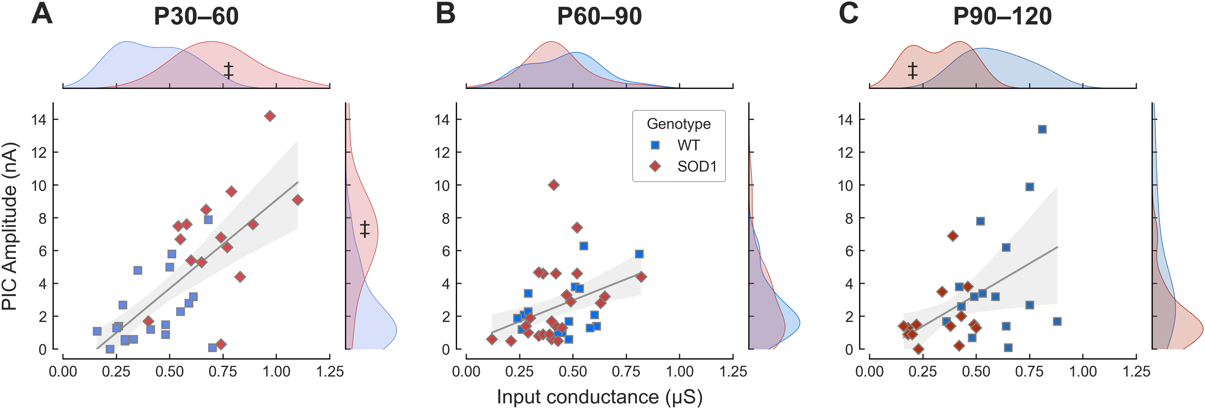
Although amyotrophic lateral sclerosis (ALS) is an adult-onset neurodegenerative disease, motoneuron electrical properties are already altered during embryonic development. Motoneurons must therefore exhibit a remarkable capacity for homeostatic regulation to maintain a normal motor output for most of the life of the patient. In the present article, we demonstrate how maintaining homeostasis could come at a very high cost. We studied the excitability of spinal motoneurons from young adult SOD1(G93A) mice to end-stage. Initially, homeostasis is highly successful in maintaining their overall excitability. This initial success, however, is achieved by pushing some cells far above the normal range of passive and active conductances. As the disease progresses, both passive and active conductances shrink below normal values in the surviving cells. This shrinkage may thus promote survival, implying the previously large values contribute to degeneration. These results support the hypothesis that motoneuronal homeostasis may be "hypervigilant" in ALS and a source of accumulating stress.

Keywords: ALS; electrophysiology; homeostasis; in vivo recording; motor neuron; spinal cord.

Figure 1.

PIC amplitude is larger is young adult mSOD1 mice. A, Example of a PIC recording from a P43 WT mouse. The green bottom trace is the ascending part of the voltage ramp. The top blue trace is the raw current. The dashed line shows the leak current estimated by fitting a straight line in the subthreshold potential region, which is used to measure the input conductance of the cell. The leak-subtracted current trace is obtained by subtracting the leak current from the raw current trace. The dash-dotted lines show some of the measurements: PIC amp.: PIC amplitude, measured at the point of largest deflection on the leak-subtracted trace; V_onset: voltage at which the PICs start to activate; V_peak: voltage at which PICs reach their maximum. B, Example of a PIC recording from a P35 mSOD1 mouse. Same organization as in A. C, Plot of the amplitude of the PICs (in nA) versus age in WT (blue square) and mSOD1 mice (red diamonds). The solid lines correspond to the linear regression lines with 95%CIs (shaded areas). WT: slope = 0.12 nA/wk 95%CI[−0.068–0.32], r² = 0.034 (p = 0.2); SOD1: slope = −0.45 nA/wk 95%CI[−0.64–−0.25], r² = 0.29 (p = 3.4e−05). D, Breakdown of the difference in PIC amplitude between WT and mSOD1 animals by age groups. P30–P60 WT: 2.30 ± 2.17 nA, N = 19 versus mSOD1: 6.73 ± 3.28 nA, N = 15; g = 1.59 95%CI[0.63–2.45]; t₍₃₂₎ = −4.50, ****p = 0.00016. P60–P90 WT: 2.47 ± 1.69 nA, N = 16 versus mSOD1: 2.75 ± 2.40 nA, N = 24; g = 0.12 95%CI[−0.53–0.65]; t₍₃₈₎ = −0.42, p = 0.67. P90–P120 WT: 4.12 ± 3.69 nA, N = 15 versus mSOD1: 1.90 ± 1.78 nA, N = 14; g = −0.74 95%CI[−1.26–0.01]; t₍₂₇₎ = 2.08, p = 0.05. E, Evolution of the membrane potential at which the PICs start to activate (PIC onset voltage) versus age. WT: slope = −0.33 mV/wk 95%CI[−0.77–0.11], r² = 0.045 (p = 0.14). SOD1: slope = 0.91 mV/wk 95%CI[0.41–1.4], r² = 0.21 (p = 0.00063). F, Evolution of the membrane potential at which the PICs reach their peak (PIC peak voltage) versus age. WT: slope = −0.29 mV/wk 95%CI[−0.73–0.16], r² = 0.034 (p = 0.2). SOD1: slope = 0.68 mV/wk 95%CI[0.28–1.1], r² = 0.18 (p = 0.0014). G, Evolution of the voltage threshold for spiking (measure in current-clamp mode) versus age. WT: slope = −0.14 mV/wk 95%CI[−0.57–0.28], r² = 0.0096 (p = 0.5). SOD1: slope = 0.77 mV/wk 95%CI[0.34–1.2], r² = 0.23 (p = 0.0007).

Figure 2.

Mutant motoneurons are not hyperexcitable. A, Example of the response of a P43 WT mouse (same motoneuron as in Fig. 1A) to a triangular ramp of current. From bottom to top, traces are: injected current, membrane potential, and instantaneous firing frequency. The dash-dotted lines show some of the measurements: I_recruit.: current intensity at which the motoneuron starts to fire; I_derecruit.: de-recruitment current; ΔI: difference between the de-recruitment and recruitment currents; I_{trans. SPR/PR}: the current at the transition between SPR and PR; F-I gain: slope of the linear fit of the firing frequency in the PR; ΔF: difference between the instantaneous firing frequency at de-recruitment and recruitment; V_th: voltage threshold for spiking measured on the first spike of the ramp. B, Example of the response of a P35 mSOD1 mouse (same motoneuron as in Fig. 1B). Same organization as in A. C, Plot of the current intensity required for eliciting the first spike on a triangular ramp of current in WT (blue squares) and mSOD1 motoneurons (red diamonds). WT: slope = 0.1 nA/wk 95%CI[−0.11–0.31], r² = 0.019 (p = 0.34). SOD1: slope = −0.35 nA/wk 95%CI[−0.56–−0.14], r² = 0.2 (p = 0.0019). D, Breakdown of the difference in recruitment current between WT and mSOD1 motoneurons in each of the age groups. In young adult and presymptomatic mice, mutant motoneurons require the same amount of current than WT motoneuron to fire, P30–P60 WT: 4.73 ± 3.14 nA, N = 19 versus mSOD1: 6.21 ± 2.51 nA, N = 14; g = 0.50 95%CI[−0.24–1.24]; t₍₃₁₎ = −1.51, p = 0.14. P60–P90 WT: 5.28 ± 2.64 nA, N = 16 versus mSOD1: 4.53 ± 3.38 nA, N = 20; g = −0.24 95%CI[−0.93–0.41]; t₍₃₄₎ = 0.75, p = 0.46. At the symptomatic stages (P90–P120), mutant motoneurons exhibit a lower current threshold for firing (WT: 5.43 ± 3.07 nA, N = 15 versus mSOD1: 2.19 ± 1.56 nA, N = 13; g = −1.26 95%CI[−1.95–−0.47]; t₍₂₆₎ = 3.59, **p = 0.0017), compatible with the loss of the least excitable cells. E, The slope of the F-I relationship, measured over the PR, is not affected by the mutation, regardless of the age of the animals. WT: slope = −0.13 Hz/nA/wk 95%CI[−0.65–0.38], r² = 0.011 (p = 0.6). SOD1: slope = 0.27 Hz/nA/wk 95%CI[−0.23–0.77], r² = 0.028 (p = 0.28). F, Breakdown of the difference between WT and mSOD1 motoneurons by age group: P30–P60 WT: 9.3 ± 3.6 Hz/nA, N = 10 versus mSOD1: 8.3 ± 3.4 Hz/nA, N = 14; g = −0.28 95%CI[−1.10–0.64]; t₍₂₂₎ = 0.69, p = 0.5. P60–P90 WT: 12.2 ± 7.3 Hz/nA, N = 8 versus mSOD1: 10.3 ± 6.4 Hz/nA, N = 16; g = −0.27 95%CI[−1.22–0.54]; t₍₂₂₎ = 0.62, p = 0.54. P90–P120 WT: 8.0 ± 3.2 Hz/nA, N = 10 versus mSOD1: 10.8 ± 9.1 Hz/nA, N = 13; g = 0.38 95%CI[−0.43–0.93]; t₍₂₁₎ = −1.04, p = 0.31.

Figure 3.

Young mutant motoneurons have an aberrantly large input conductance. A, Plot of the motoneuron input conductance versus age in WT (blue squares) and mSOD1 (red diamonds) animals. The solid lines correspond to the linear regression lines with 95%CIs (shaded areas). WT slope = 0.018 μS/wk 95%CI[0.0061–0.029], r² = 0.16 (p = 0.0035); SOD1 slope = −0.041 μS/wk 95%CI[−0.052–−0.03], r² = 0.53 (p = 6.1e−10).) B, Breakdown of the difference in input conductance between WT and mSOD1 animals by age groups. P30–P60 WT: 0.42 ± 0.16 μS, N = 19 versus mSOD1: 0.72 ± 0.18 μS, N = 15; g = 1.73 95%CI[0.92–2.41]; t₍₃₂₎ = −5.06, ****p = 2.2e−05. P60–P90 WT: 0.46 ± 0.16 μS, N = 16 versus mSOD1: 0.42 ± 0.15 μS, N = 24; g = −0.28 95%CI[−0.96–0.37]; t₍₃₈₎ = 0.88, p = 0.39. P90–P120 WT: 0.60 ± 0.15 μS, N = 15 versus mSOD1: 0.33 ± 0.13 μS, N = 14; g = −1.85 95%CI[−2.57–−1.16]; t₍₂₇₎ = 5.16, ****p = 2.1e−05.

Figure 4.

The RMP of young adult mutant mice is hyperpolarized. A, Plot of the motoneuron RMP versus age in WT (blue squares) and mSOD1 (red diamonds) animals. The solid lines correspond to the linear regression lines with 95%CIs (shaded areas). WT: slope = −0.068 mV/wk 95%CI[−0.52–0.38], r² = 0.0019 (p = 0.76). SOD1: slope = 0.81 mV/wk 95%CI[0.31–1.3], r² = 0.18 (p = 0.0022). B, Breakdown of the difference in RMP between WT and mSOD1 animals by age groups. P30–P60 WT: −62.38 ± 5.52 mV, N = 19 versus mSOD1: −71.45 ± 8.78 mV, N = 15; g = −1.24 95%CI[−2.13–−0.23]; t₍₃₂₎ = 3.49, ***p = 0.002. P60–P90 WT: −60.98 ± 5.35 mV, N = 16 versus mSOD1: −66.18 ± 5.63 mV, N = 22; g = −0.92 95%CI[−1.54–−0.18]; t₍₃₆₎ = 2.89, **p = 0.0067. P90–P120 WT: −64.71 ± 7.42 mV, N = 15 versus mSOD1: −61.99 ± 5.43 mV, N = 13; g = 0.40 95%CI[−0.35–1.10]; t₍₂₆₎ = −1.12, p = 0.27.

Figure 5.

Some motoneurons exhibit properties outside of the normal range. A, Plot of the PIC amplitude versus the input conductance of young adult motoneurons (P30–P60) in WT (blue squares) and mSOD1 (red diamonds) animals. The gray line is the best linear fit ± 95%CI (shaded area) for both samples. Slope = 7.7 mV 95%CI[2.6–12.7], r² = 0.55 (p = 0.004). The marginal plots indicate the kernel density estimation of the distributions of the values in the two populations. The ‡ symbol points to the fraction of the mSOD1 population that is outside the range of the WT population. B, Same as A for the presymptomatic age range P60–P90. Slope = 5.4 mV 95%CI[1.1–9.8], r² = 0.15 (p = 0.016). C, Same as A for the symptomatic age range P90–P120. Slope = 7.0 mV 95%CI[−0.8–14.9], r² = 0.23 (p = 0.078).

Figure 6.

Some cells are hypoexcitable and cannot fire repetitively. A, Example of an mSOD1 motoneuron (from a P88 mouse) that is unable to fire repetitively in response to a triangular ramp of current. Top trace, Membrane potential. Bottom trace, Injected current. B, This same motoneuron was nevertheless able to generate a single full-height AP in response to a square pulse of current. Same organization as in A. C, Voltage-clamp measurement of the PICs in this same motoneuron. Traces are (from top to bottom), leak current (dashed line), raw current (blue), leak-subtracted current (red), and voltage command (green). D, Non-firing motoneurons had a similar input conductance compared with motoneurons capable of firing repetitively. Firing: 0.49 ± 0.22 μS, N = 47 versus non-firing: 0.38 ± 0.20 μS, N = 6; g = −0.54 95%CI[−1.11–0.50]; t₍₅₁₎ = 1.36, p = 0.22. E, Non-firing motoneurons had much smaller PICs than motoneurons able to fire repetitively. Firing: 4.04 ± 3.18 nA, N = 47 versus non-firing: 0.60 ± 0.49 nA, N = 6; g = −1.12 95%CI[−1.42–−0.86]; t₍₅₁₎ = 6.81, ****p = 1.3e−08. F, Non-firing motoneurons appear earlier in mSOD1 animals compared with WT animals. WT: 100 ± 16 d old, N = 7 versus SOD1: 75 ± 23 d old, N = 6; g = −1.20 95%CI[−2.06–0.01]; t₍₁₁₎ = 2.24, p = 0.053.

Figure 7.

Overview of the change in PCs over time. A_1–A₃, Plot of the three first PCs versus age in WT (blue squares) and mSOD1 motoneurons (red diamonds). The solid lines correspond to the linear regression lines with 95%CIs (shaded areas). B, Heatmap showing the correlation coefficient between each PC (columns) and the features (rows) shown on the right. Correlation coefficients are color-coded from dark blue (r = −1) to dark red (r = +1). C, Summary of the evolution of the difference between WT and mSOD1 motoneurons (quantified by the effect size Hedges’ g) for each of the features and each of the time points considered. The features are ordered by the size of the effect of the mutation in the P30–P60 age group. On each row, the dashed line represents an effect size of zero. Scale bar: 2 units.

Figure 8.

summary of the changes in motoneuron properties over time. Schematic representation of the changes in four key electrophysiological properties over time. The dots represent the effect size (Hedges’ g) and the vertical bars show the 95%CI around g. The thin lines are cubic splines interpolation of the data over time. The points have been slightly staggered so that the vertical bars do not occlude each other. †Data from embryonic motoneurons are from Martin et al. (2013). These authors did not measure PICs in embryonic motoneurons. Kuo et al. (2004) did measure PICs, but their embryonic motoneurons were cultured for 10–30 d in vitro, and their development stage is therefore uncertain. ‡Data from neonates (P0–P5 and P6–P12) are from Quinlan et al. (2011).

References

1. Attwell D, Laughlin SB (2001) An energy budget for signaling in the grey matter of the brain. J Cereb Blood Flow Metab 21:1133–1145. 10.1097/00004647-200110000-00001 - DOI - PubMed
1. Bączyk M, Ouali Alami N, Delestrée N, Martinot C, Tang L, Commisso B, Bayer D, Doisne N, Frankel W, Manuel M, Roselli F, Zytnicki D (2020) Synaptic restoration by cAMP/PKA drives activity-dependent neuroprotection to motoneurons in ALS. J Exp Med 217:e20191734. - PMC - PubMed
1. Bernard C (2019) Changing the way we report, interpret, and discuss our results to rebuild trust in our research. eNeuro 6:ENEURO.0259-19.2019. 10.1523/ENEURO.0259-19.2019 - DOI - PMC - PubMed
1. Bhumbra GS, Beato M (2018) Recurrent excitation between motoneurones propagates across segments and is purely glutamatergic. PLoS Biol 16:e2003586. 10.1371/journal.pbio.2003586 - DOI - PMC - PubMed
1. Brownstone RM, Lancelin C (2018) Escape from homeostasis: spinal microcircuits and progression of amyotrophic lateral sclerosis. J Neurophysiol 119:1782–1794. 10.1152/jn.00331.2017 - DOI - PMC - PubMed