Sustained neural rhythms reveal endogenous oscillations supporting speech perception

Abstract

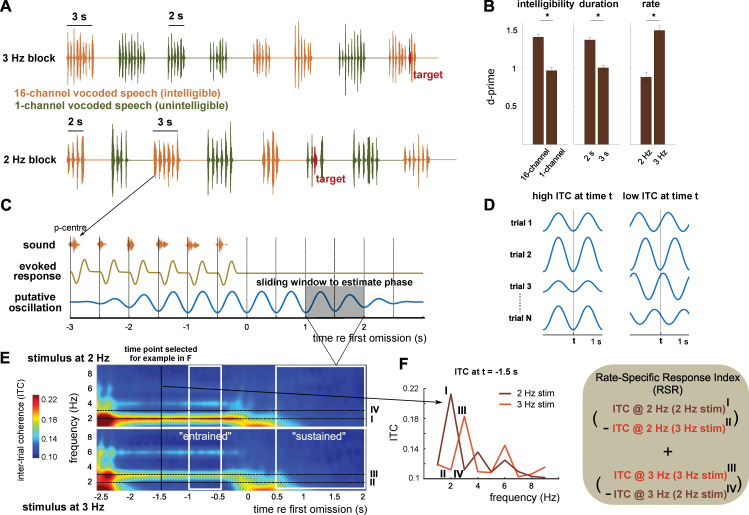
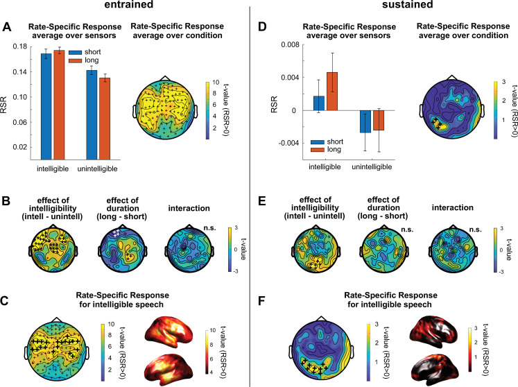
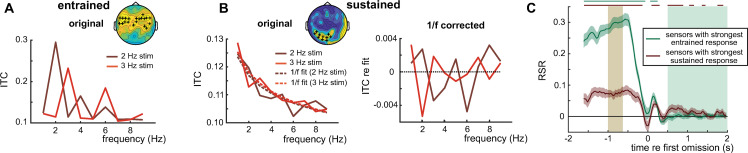
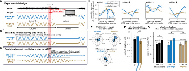
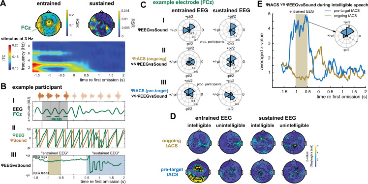
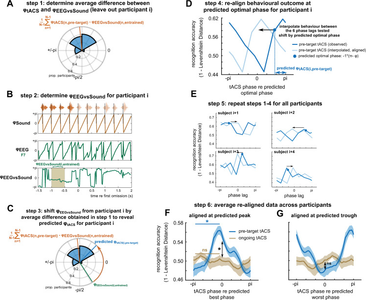
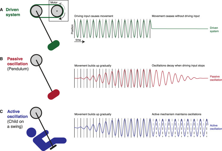
Rhythmic sensory or electrical stimulation will produce rhythmic brain responses. These rhythmic responses are often interpreted as endogenous neural oscillations aligned (or "entrained") to the stimulus rhythm. However, stimulus-aligned brain responses can also be explained as a sequence of evoked responses, which only appear regular due to the rhythmicity of the stimulus, without necessarily involving underlying neural oscillations. To distinguish evoked responses from true oscillatory activity, we tested whether rhythmic stimulation produces oscillatory responses which continue after the end of the stimulus. Such sustained effects provide evidence for true involvement of neural oscillations. In Experiment 1, we found that rhythmic intelligible, but not unintelligible speech produces oscillatory responses in magnetoencephalography (MEG) which outlast the stimulus at parietal sensors. In Experiment 2, we found that transcranial alternating current stimulation (tACS) leads to rhythmic fluctuations in speech perception outcomes after the end of electrical stimulation. We further report that the phase relation between electroencephalography (EEG) responses and rhythmic intelligible speech can predict the tACS phase that leads to most accurate speech perception. Together, we provide fundamental results for several lines of research-including neural entrainment and tACS-and reveal endogenous neural oscillations as a key underlying principle for speech perception.

Fig 1. Experimental paradigm and analysis.

(A) Participants listened to rhythmic speech sequences and were asked to press a button when they detected an irregularity in the stimulus rhythm (red targets). (B) Performance (as d-prime) in the irregularity detection task, averaged across participants and shown for the main effects of intelligibility, duration, and rate. Error bars show SEM, corrected for within-subject comparison [19]. Please refer to S1 Data for the numerical values underlying this figure panel. (C) A rhythmic brain response measured during the presented sounds cannot distinguish true neural oscillations aligned to the stimulus from regular stimulus-evoked responses. However, only the oscillation-based model predicts a rhythmic response which outlasts the rhythmic stimulus. For each time point t throughout the trial, oscillatory phase was estimated based on a 1-second window centred on t (shaded grey). (D) ITC at time t is high when estimated phases are consistent across trials (left) and low otherwise (right). Note that the 2 examples shown differ in their 2-Hz ITC, but have similar induced power at the same frequency. (E) ITC in the longer (3-second) condition, averaged across intelligibility conditions, gradiometers, and participants. Note that “time” (x-axis) refers to the centre of the 1-second windows used to estimate phase. ITC at 2 and 3 Hz, measured in response to 2 and 3 Hz sequences, were combined to form an RSR. The 2 time windows used for this analysis (“entrained” and “sustained”) are shown in white (results are shown in Fig 2). (F) ITC as a function of neural frequency, separately for the 2 stimulation rates, and for the example time point shown as a black line in E. ITC, intertrial phase coherence; RSR, rate-specific response; SEM, standard error of mean.

Fig 2. Main results from Experiment 1.

(A–C) Results in the entrained time window. Bars in panel A show RSR in the different conditions, averaged across gradiometers and participants. Error bars show SEM, corrected for within-subject comparison. The topography shows t-values for the comparison with 0, separately for the 102 gradiometer pairs, and after RSR was averaged across conditions. Topographies in B contrast RSR across conditions. Topography and source plots in C show t-values for the comparison with 0 in the intelligible conditions. In all topographic plots, plus signs indicate the spatial extent of significant clusters from cluster-based permutation tests (see Materials and methods). In B, white plus signs indicate a cluster with negative polarity (i.e., negative t-values) for the respective contrast. In A and C, this cluster includes all gradiometers (small plus signs). In C, larger plus signs show the 20 sensors with the highest RSR, selected for subsequent analyses (Fig 3). (D–F) Same as A–C, but for the sustained time window. Please refer to S1 Data for the numerical values underlying this figure. RSR, rate-specific response; SEM, standard error of mean.

Fig 3. Follow-up analyses from Experiment 1, using selected sensors (plus signs in insets, reproducing Fig 2C and 2F, respectively).

(A, B) ITC as a function of neural frequency, measured during (A) and after (B) intelligible speech, presented at 2 and 3 Hz. Note that these ITC values were combined to form RSR shown in Fig 2, as described in Fig 1F. For the right panel in B, a fitted “1/f” curve (shown as dashed lines in the left panel) has been subtracted from the data (see Materials and methods). Note that the peaks correspond closely to the respective stimulus rates, or their harmonics (potentially produced by imperfect sinusoidal signals). (C) RSR during intelligible speech as a function of time, for the average of selected sensors. Horizontal lines on top of the panel indicate an FDR-corrected p-value of < = 0.05 (t test against 0) for the respective time point and sensor group. Shaded areas correspond to the 2 defined time windows (brown: entrained, green: sustained). Shaded areas around the curves show SEM. Please refer to S1 Data for the numerical values underlying this figure. FDR, false discovery rate; ITC, intertrial phase coherence; RSR, rate-specific response; SEM, standard error of mean.

Fig 4. Experimental paradigm and main results from Experiment 2.

(A) Experimental paradigm. In each trial, a target word (red), embedded in noise (black), was presented so that its p-centre falls at 1 of 6 different phase lags (vertical red lines; the thicker red line corresponds to the p-centre of the example target), relative to preceding (“pretarget tACS”) or ongoing tACS (which was then turned off). After each trial, participants were asked to type in the word they had heard. The inset shows the electrode configuration used for tACS in both conditions. (B, C). Theoretical predictions. (B) In the case of entrained neural activity due to tACS, this would closely follow the applied current and hence modulate perception of the target word only in the ongoing tACS condition. (C) In the case that true oscillations are entrained by tACS, these would gradually decay after tACS offset, and a “rhythmic entrainment echo” might therefore be apparent as a sustained oscillatory effect on perception even in the pretarget condition. (D) Accuracy in the word report task as a function of phase lag (relative to tACS peak shown in (A), averaged across tACS durations, and for 4 example participants. Phasic modulation of word report was quantified by fitting a cosine function to data from individual participants (dashed lines). The amplitude (a) of this cosine reflects the magnitude of the hypothesized phasic modulation. The phase of this cosine (φ_tACS) reflects the distance between its peak and the maximal phase lag of π. Note that the phase lag with highest accuracy for the individual participants, estimated based on the cosine fit, therefore corresponds to π-φ_tACS. (E) Distribution of φ_tACS in the 2 tACS conditions, and their difference. (F, G) Amplitudes of the fitted cosines (cf. amplitude a in panel D), averaged across participants. In (F), cosine functions were fitted to data averaged over tACS duration (cf. panel D). In (G), cosine functions were fitted separately for the 3 durations. For the black bars, cosine amplitudes were averaged across the 2 tACS conditions. Dashed lines show the threshold for statistical significance (p < = 0.05) for a phasic modulation of task accuracy, obtained from a surrogate distribution (see Materials and methods). Error bars show SEM (corrected for within-subject comparisons in (F)). Please refer to S1 Data for the numerical values underlying panels E–G. n.s., not significant; SEM, standard error of mean; tACS, transcranial alternating current stimulation.

Fig 5. Combining Experiments 1 and 2.

(A) EEG results from Experiment 1. Topographies show RSR in the intelligible conditions. The time–frequency representation depicts ITC during 3-Hz sequences, averaged across EEG electrodes, participants, and conditions (cf. Fig 1C). (B) Illustration of methodological approach, using example data from 1 participant and electrode (FCz, green in panel A). (B-I) Band-pass filtered (2–4 Hz) version of the EEG signal that has been used to estimate φ_EEG in the panel below (B-II). In practice, EEG phase at 3 Hz was estimated using FFT applied to unfiltered EEG data. Consequently, φ_EEG reflects the distance between the peaks of a cosine, fitted to data within the analysis window (shaded grey), and the end of each 3-Hz cycle (green arrows). (B-II) φ_EEG (green; in the intelligible conditions and averaged across durations) and phase of the 3-Hz sequence (φ_Sound, orange). The latter is defined so that the perceptual centre of each word corresponds to phase π (see example sound sequence, and its theoretical continuation, on top of panel B-I). (B-III) Circular difference between φ_EEG (green in B-II) and φ_Sound (orange in B-II), yielding φ_EEGvsSound. Given that φ is defined based on a cosine, a positive difference means that EEG lags sound. (C) Distribution of individual φ_EEGvsSound, and its relation to φ_tACS. Data from 1 example electrode (FCz) is used to illustrate the procedure; main results and statistical outcomes are shown in panel D. (C-I) Distribution of φ_EEGvsSound (cf. B-III), extracted in the intelligible conditions, and averaged across durations and within the respective time windows (shaded brown and blue in B-III, respectively). (C-II,III) Distribution of the circular difference between φ_tACS (Fig 4E) and φ_EEGvsSound (C-I). Note that a nonuniform distribution (tested in panel D) indicates a consistent lag between individual φ_tACS and φ_EEGvsSound. (D) Z-values (obtained by means of a Rayleigh test; see Materials and methods), quantifying nonuniformity of the distributions shown in C-II,III for different combinations of experimental conditions. Plus signs show electrodes selected for follow-up analyses (FDR-corrected p < = 0.05). (E) Z-values shown in D for intelligible conditions as a function of time, averaged across selected EEG sensors (plus signs in D). For the electrode with the highest predictive value for tACS (F3), the inset shows the distribution of the circular difference between φ_tACS and φ_EEGvsSound in the pretarget condition, averaged within the entrained time window (shaded brown). Please refer to S1 Data for the numerical values underlying panels A, C–E. EEG, electroencephalography; FDR, false discovery rate; FFT, fast Fourier transformation; ITC, intertrial phase coherence; RSR, rate-specific response; tACS, transcranial alternating current stimulation.

Fig 6. Predicted individual preferred tACS phases in the pretarget tACS condition from EEG data measured in the entrained time window at sensor F3.

(A) Step 1: For each participant i, data from all remaining participants were used to estimate the average difference between φ_tACS and φ_EEGvsSound. (B) Step 2: φ_EEGvsSound was determined for participant i. (C) Step 3: This φ_EEGvsSound was shifted by the phase difference obtained in step 1, yielding the predicted φ_tACS for participant i. (D) Step 4: The predicted φ_tACS was used to estimate the tACS phase lag with highest perceptual accuracy for participant i, and the corresponding behavioural data were shifted so that highest accuracy was located at a centre phase bin. Prior to this step, the behavioural data measured at the 6 different phase lags were interpolated to enable realignment with higher precision. (E) Step 5: This procedure was repeated for all participants. (F) Step 6: The realigned data were averaged across participants (blue). For comparison, the procedure was repeated for the ongoing tACS condition (using EEG data from the same sensor; brown). The shaded areas show SEM, corrected for within-subject comparison. (G). Same as in (F), but aligned at the predicted worst phase for word report accuracy. Please refer to S1 Data for the numerical values underlying panels F and G. EEG, electroencephalography; SEM, standard error of mean; tACS, transcranial alternating current stimulation.

Fig 7. Three physical models that could be invoked to explain neural entrainment, and their potential to explain rhythmic entrainment echoes.

(A) In a system without any endogenous processes (e.g., neural oscillations), driving input would produce activity which ceases immediately when this input stops. (B) A more direct account of rhythmic entrainment echoes is that endogenous neural oscillations resemble the operation of a pendulum which will start swinging passively when “pushed” by a rhythmic stimulus. When this stimulus stops, the oscillation will persist but decays over time, depending on certain “hard-wired” properties (similar to the frictional force and air resistance that slows the movement of a pendulum over time). (C) Endogenous neural oscillations could include an active (e.g., predictive) component that controls a more passive process—similar to a child that can control the movement of a swing. This model predicts that oscillations are upheld after stimulus offset as long as the timing of important upcoming input (dashed lines) can be predicted. Note that, for the sake of clarity, we made extreme predictions to illustrate the different models. For instance, depending on the driving force of the rhythmic input, pendulum and swing could reach their maximum amplitude near-instantaneously in panels B and C, respectively, and therefore initially resemble the purely driven system shown in A. Similarly, it is possible that the predictive process (illustrated in C) operates less efficiently in the absence of driving input and therefore shows a decay similar to that shown by the more passive process (shown in B).

References

1. Giraud A-L, Poeppel D. Cortical oscillations and speech processing: emerging computational principles and operations. Nat Neurosci. 2012;15:511–7. 10.1038/nn.3063 - DOI - PMC - PubMed
1. Ding N, Melloni L, Zhang H, Tian X, Poeppel D. Cortical tracking of hierarchical linguistic structures in connected speech. Nat Neurosci. 2016;19:158–64. 10.1038/nn.4186 - DOI - PMC - PubMed
1. Peelle JE, Davis MH. Neural Oscillations Carry Speech Rhythm through to Comprehension. Front Psychol. 2012;3:320. 10.3389/fpsyg.2012.00320 - DOI - PMC - PubMed
1. Zoefel B, VanRullen R. The Role of High-Level Processes for Oscillatory Phase Entrainment to Speech Sound. Front Hum Neurosci. 2015;9:651. 10.3389/fnhum.2015.00651 - DOI - PMC - PubMed
1. Peelle JE, Gross J, Davis MH. Phase-locked responses to speech in human auditory cortex are enhanced during comprehension. Cereb Cortex. 2013;23:1378–87. 10.1093/cercor/bhs118 - DOI - PMC - PubMed
Publication types