Reacting to outbreaks at neighboring localities

Abstract

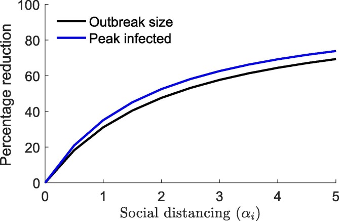
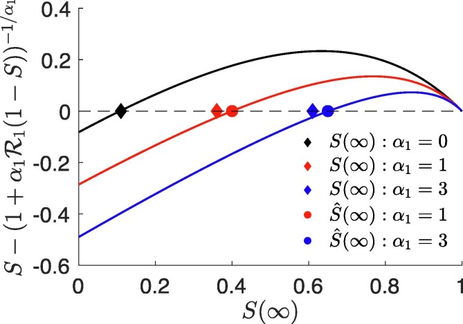
We study the dynamics of epidemics in a networked metapopulation model. In each subpopulation, representing a locality, the disease propagates according to a modified susceptible-exposed-infected-recovered (SEIR) dynamics. In the modified SEIR dynamics, individuals reduce their number of contacts as a function of the weighted sum of cumulative number of cases within the locality and in neighboring localities. We consider a scenario with two localities where disease originates in one locality and is exported to the neighboring locality via travel of exposed (latently infected) individuals. We establish a lower bound on the outbreak size at the origin as a function of the speed of spread. Using the lower bound on the outbreak size at the origin, we establish an upper bound on the outbreak size at the importing locality as a function of the speed of spread and the level of preparedness for the low mobility regime. We evaluate the critical levels of preparedness that stop the disease from spreading at the importing locality. Finally, we show how the benefit of preparedness diminishes under high mobility rates. Our results highlight the importance of preparedness at localities where cases are beginning to rise such that localities can help stop local outbreaks when they respond to the severity of outbreaks in neighboring localities.

Keywords: Epidemiology; Networked metapopulation; Nonlinear dynamics; Social distancing.

Fig. 1

Networked SEIR model with no-distancing. Two localities are connected with travel rates ${\lambda }_{\mathit{ij}}\in \{1\%,0.01\%,0.001\%\}$. The disease propagates in both localities according to SEIR dynamics with no response to disease prevalence, i.e., ${\alpha }_i=0$. Blue and red lines show the ratio of susceptible and infected individuals in a locality, respectively. The differences in time of peaks are 10, 38, 51 days respectively for ${\lambda }_{\mathit{ij}}\in \{1\%,0.01\%,0.001\%\}$. Final outbreak sizes of localities 1 and 2 are almost identical for low mobility regimes.

Fig. 2

Percentage reduction in outbreak size and ratio of infected at peak with respect to increasing social distancing exponent (${\alpha }_i$). We measure the reduction with respect to the no-distancing case (${\alpha }_i=0$). In both cases, the mobility per day is ${\lambda }_{12}={\lambda }_{21}=0.001\%$ of the population.

Fig. 3

Upper bound values of $S\left(\infty \right)$ obtained by solving (6) for $k=1$ and $k=3$. We let ${\mathcal{N}}_1=2.5$. Lines correspond to the left hand side of (6). Circle dots show the solution to (6). Diamond dots are $S\left(\infty \right)$ values obtained by simulating the SEIR model in (1)–(4) with ${\beta }_i$ given in (5). For $k=0$, we use standard speed-size relations for the SEIR model without social distancing (Ma and Earn, 2006). Note that the relation for the standard SEIR model is exact. Thus, diamond and circle dots overlap for $k=0$. The difference between the upper bound for $S\left(\infty \right)$ ($\widehat{S}\left(\infty \right)$) and the simulated $S\left(\infty \right)$ is relatively constant for different values of ${\alpha }_1$.

Fig. 4

Outbreak size at Locality 2 with respect to adopted awareness ${\omega }_{21}$. (Top) Weak (${\alpha }_2=1$) and (Bottom) Strong (${\alpha }_2=3$) responses at Locality 2. Mobility is set to $\lambda =0.001\%$. Weak and strong responses at Locality 1 correspond to ${\alpha }_1=1$ (black) and ${\alpha }_1=3$ (blue), respectively. The outbreak size at Locality 2 decreases with increasing adopted awareness values. The decrease is sharper when response at the origin is weak. Corresponding theoretical upper bound values (shown by dashed lines) are tighter at larger adopted awareness values. In the Bottom figure, the critical threshold values ${\omega }_{21}^{\ast }$ above which disease does not propagate approximately equal to 0.5 and 0.8 respectively for weak (black) and strong (blue) responses at the origin. (For interpretation of the references to colour in this figure legend, the reader is referred to the web version of this article.)

Fig. 5

Total of outbreak sizes at localities 1 and 2 with respect to adopted awareness ${\omega }_{21}$. (Top) Weak (${\alpha }_2=1$) and (Bottom) strong (${\alpha }_2=3$) responses at Locality 2. Mobility is set to $\lambda =0.001\%$. Weak and strong response at Locality 1 correspond to (${\alpha }_1=1$) and (${\alpha }_1=3$), respectively. There exists a critical adopted awareness constant value in Top where the total outbreak size is lower in the scenario where both localities respond weakly compared to the scenario where Locality 1 has a strong response. The critical value for the adopted awareness constant value can be found by looking at the intersection of the solid black line with the solid blue line for the corresponding mobility value. When both localities respond strongly to the disease in Bottom figure, such a critical adopted awareness constant value does not exist.

Fig. 6

Benefit of adopted awareness with respect to mobility rates. (Top) Weak and (Bottom) strong responses at the origin. The strength of response at Locality 2 is weak ${\alpha }_2=1$. The benefit is measured as the reduction in final size with respect to the zero-adopted awareness constant scenario ${\omega }_{21}=0$. Let $F_2({\omega }_{21},{\lambda }_{12})$ denote the final outbreak size at Locality 2 with respect to ${\omega }_{21}$ and ${\lambda }_{12}$. The benefit of alertness is defined as $F_2(0,{\lambda }_{12})-F_2({\omega }_{21},{\lambda }_{12})$. Weak response at the origin, higher adopted awareness leads a smaller outbreak size at Locality 2 (Top). Given a strong response at the origin, higher adopted awareness can lead to higher outbreak sizes (Bottom). Strong response at the origin reduces the magnitude of the benefit of adopted awareness.

Fig. S1

Lower bound values for $S\left(\infty \right)$. We assume low adopted awareness ${\omega }_{21}=1/2$. We let ${\mathcal{R}}_1=2.5$ and $\lambda =0.0001\%$. (Top) Weak and (Bottom) strong response at the origin. Lines correspond to the left hand side of (10). Circle dots show the solution to (10), i.e., intersection of lines with zero. Diamond dots are $S\left(\infty \right)$ values obtained by simulating the SEIR model in (1)–(4) with ${\beta }_i$ in (5).

Fig. S2

Lower bound values for $S\left(\infty \right)$. We assume high adopted awareness ${\omega }_{21}=3/4$. We let ${\mathcal{R}}_1=2.5$ and $\lambda =0.0001\%$. (Top) Weak and (Bottom) strong response at the origin. Lines correspond to the left hand side of (10). Circle dots show the solution to (10), i.e., intersection of lines with zero. Diamond dots are $S\left(\infty \right)$ values obtained by simulating the SEIR model in (1)–(4) with ${\beta }_i$ in (5).

Fig. S3

(Left) Population size and mobility flow changes over time. Left y-axis shows the population sizes of localities. Right y-axis shows relative mobility flow from locality 1 to locality 2 over time. (Right) Outbreak size at Locality 2. The flow ${\lambda }_{12}\left(t\right)$ is as given in (C.1) with $\kappa =5$. The rest of the parameters of the model (1)–(4) are ${\beta }_0=5/8,\mu =1/3,\delta =1/4$, and ${\lambda }_{12}=0.001\%,N_1=N_2=1,{\alpha }_1={\alpha }_2=1$ and ${\omega }_{21}=0.5$.

Fig. S4

Outbreak size at locality 2 as a function of the population size ratio. Population size ratio is given by the ratio of initial population sizes between localities, i.e., $N_1/N_2$. The epidemic and mobility dynamics are given by (1)–(4) and Eq. (5) in the revised manuscript. Parameters: ${\beta }_0=5/8,\mu =1/3,\delta =1/4,{\lambda }_{12}={\lambda }_{21}={10}^{-7}$, and ${\alpha }_1={\alpha }_2=1$.

Fig. S5

Benefit of adopted awareness versus the change in peak times as the infection rate changes. We let ${\beta }_0\in [0.5,0.75]$. The peak time difference is the difference between the time Locality 2 peaks and the time Locality 1 peaks. Let $F_2({\omega }_{21},\mathrm{\Delta }\beta )$ denote the final outbreak size at Locality 2 with respect to ${\omega }_{21}$ and $\mathrm{\Delta }\beta$. The benefit of awareness is defined as $F_2(0,\mathrm{\Delta }\beta )-F_2({\omega }_{21},\mathrm{\Delta }\beta )$ where $\mathrm{\Delta }\beta \in [-0.125,0.125]$. Parameters of the dynamics (1)–(5): $\mu =1/3,\delta =1/4,N_1=N_2=1,{\alpha }_1={\alpha }_2=1$, and ${\lambda }_{12}={\lambda }_{21}={10}^{-5}$.

References

1. Bairagi A.K., Masud M., Munir M.S., Nahid A.-A., Abedin S.F., Alam K.M., Biswas S., Alshamrani S.S., Han Z., Hong C.S., et al. Controlling the outbreak of covid-19: A noncooperative game perspective. IEEE Access. 2020;8:215570–215581. - PMC - PubMed
1. Baker R.E., Park S.W., Yang W., Vecchi G.A., Metcalf C.J.E., Grenfell B.T. The impact of covid-19 nonpharmaceutical interventions on the future dynamics of endemic infections. Proc. Nat. Acad. Sci. 2020;117(48):30547–30553. - PMC - PubMed
1. Chinazzi M., Davis J.T., Ajelli M., Gioannini C., Litvinova M., Merler S., y Piontti A.P., Mu K., Rossi L., Sun K., et al. The effect of travel restrictions on the spread of the 2019 novel coronavirus (COVID-19) outbreak. Science. 2020;368(6489):395–400. - PMC - PubMed
1. Chiu W.A., Fischer R., Ndeffo-Mbah M.L. State-level needs for social distancing and contact tracing to contain COVID-19 in the United States. Nat. Human Behav. 2020;4(10):1080–1090. - PMC - PubMed
1. Colizza V., Vespignani A. Invasion threshold in heterogeneous metapopulation networks. Phys. Rev. Lett. 2007;99(14) - PubMed
Publication types
LinkOut - more resources