Opportunistic Screening at Abdominal CT: Use of Automated Body Composition Biomarkers for Added Cardiometabolic Value
- PMID: 33646902
- PMCID: PMC7924410
- DOI: 10.1148/rg.2021200056
Opportunistic Screening at Abdominal CT: Use of Automated Body Composition Biomarkers for Added Cardiometabolic Value
Abstract
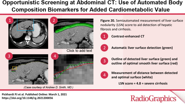
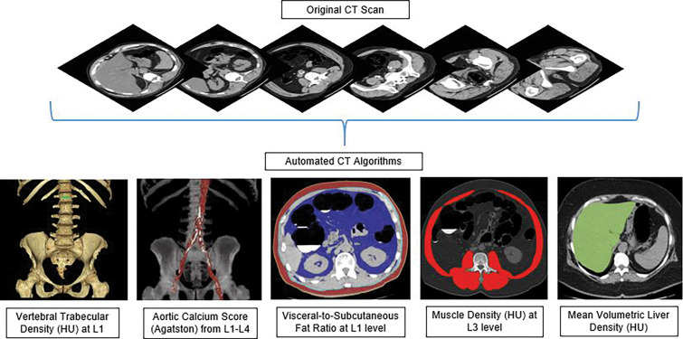
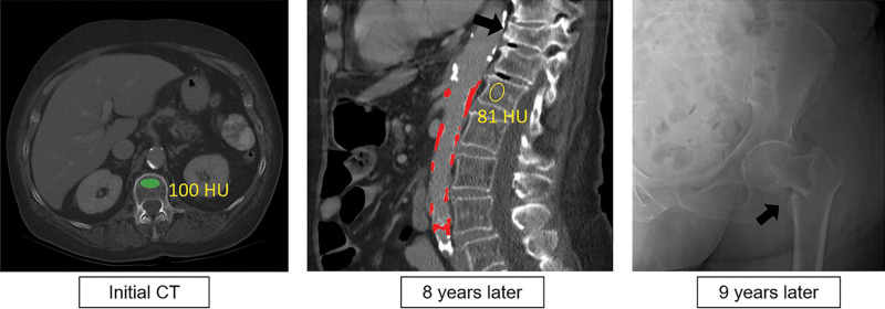
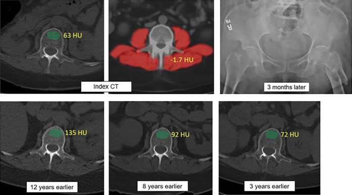
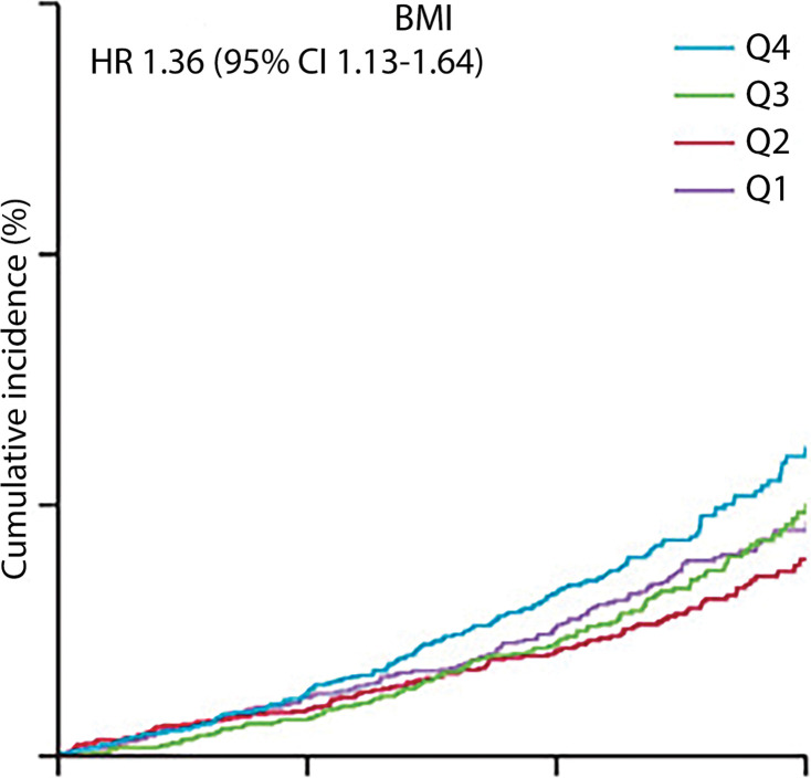
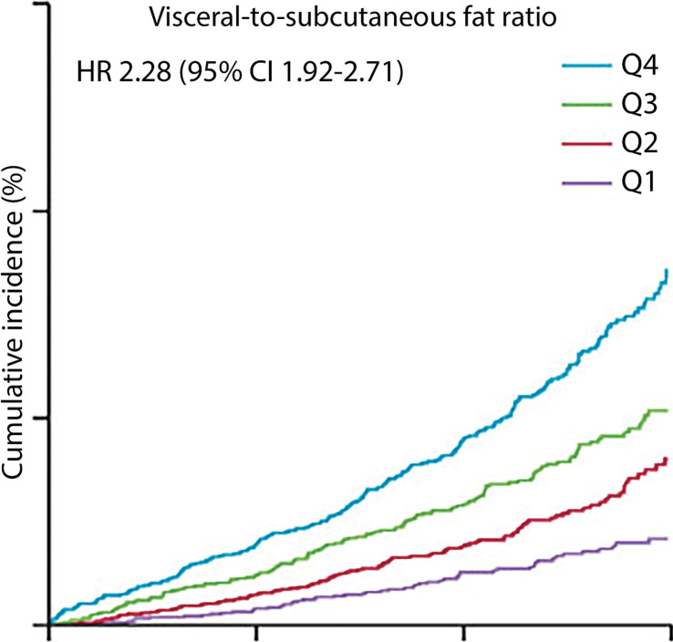
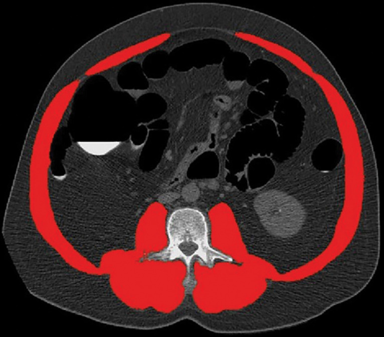
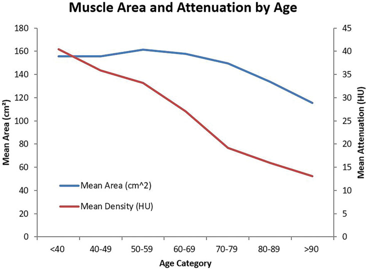
Abdominal CT is a frequently performed imaging examination for a wide variety of clinical indications. In addition to the immediate reason for scanning, each CT examination contains robust additional data on body composition that generally go unused in routine clinical practice. There is now growing interest in harnessing this additional information. Prime examples of cardiometabolic information include measurement of bone mineral density for osteoporosis screening, quantification of aortic calcium for assessment of cardiovascular risk, quantification of visceral fat for evaluation of metabolic syndrome, assessment of muscle bulk and density for diagnosis of sarcopenia, and quantification of liver fat for assessment of hepatic steatosis. All of these relevant biometric measures can now be fully automated through the use of artificial intelligence algorithms, which provide rapid and objective assessment and allow large-scale population-based screening. Initial investigations into these measures of body composition have demonstrated promising performance for prediction of future adverse events that matches or exceeds the best available clinical prediction models, particularly when these CT-based measures are used in combination. In this review, the concept of CT-based opportunistic screening is discussed, and an overview of the various automated biomarkers that can be derived from essentially all abdominal CT examinations is provided, drawing heavily on the authors' experience. As radiology transitions from a volume-based to a value-based practice, opportunistic screening represents a promising example of adding value to services that are already provided. If the potentially high added value of these objective CT-based automated measures is ultimately confirmed in subsequent investigations, this opportunistic screening approach could be considered for intentional CT-based screening. ©RSNA, 2021.
Figures
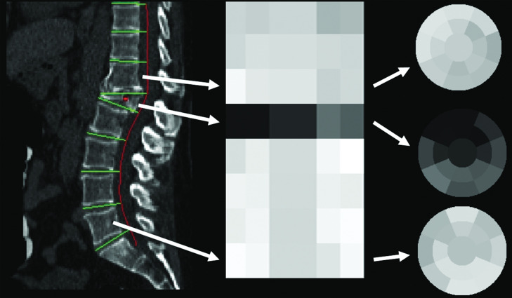
![(a) CT-based assessment of bone mineral density with the use of trabecular attenuation at the L1 vertebral level. Axial CT images show the L1 vertebral level (top row) in adult patients of a variety of ages. Magnified axial CT views show the L1 vertebra in soft tissue (second row) and bone (third row) windows. Standard manual placement of the ROI for measurement of trabecular attenuation and the mean attenuation value in the ROI are shown in the third row. Automated ROI placement was programmed to match this location. Sagittal reconstruction images (bottom row, soft-tissue [left] and bone [right] windows) show placement of the ROI (yellow oval) at the L1 vertebra. Typically, trabecular attenuation values progressively decrease with increasing patient age. The loss of bone mineral density is more apparent with the soft-tissue window. (Reprinted, with permission, from reference 39.) (b) Graph (left) shows normative reference CT-based L1 trabecular attenuation values based on more than 20 000 examinations. The mean attenuation values show that age-related L1 trabecular bone loss is fairly linear. Error bars indicate standard deviations, which are remarkably uniform throughout the age spectrum. Table (right) shows the median and the mean (± standard deviation [SD] ) values for L1 trabecular attenuation for each age group. These normative reference ranges, which are derived from a combination of manual and automated measurements, can serve as a quick reference for radiologists when reading body CT examinations performed for other clinical indications. Note that these values apply to scanning at 120 kVp. (Reprinted, with permission, from reference 37.)](https://cdn.ncbi.nlm.nih.gov/pmc/blobs/2101/7924410/bb466112f919/rg.2021200056.fig2a.jpg)
![(a) CT-based assessment of bone mineral density with the use of trabecular attenuation at the L1 vertebral level. Axial CT images show the L1 vertebral level (top row) in adult patients of a variety of ages. Magnified axial CT views show the L1 vertebra in soft tissue (second row) and bone (third row) windows. Standard manual placement of the ROI for measurement of trabecular attenuation and the mean attenuation value in the ROI are shown in the third row. Automated ROI placement was programmed to match this location. Sagittal reconstruction images (bottom row, soft-tissue [left] and bone [right] windows) show placement of the ROI (yellow oval) at the L1 vertebra. Typically, trabecular attenuation values progressively decrease with increasing patient age. The loss of bone mineral density is more apparent with the soft-tissue window. (Reprinted, with permission, from reference 39.) (b) Graph (left) shows normative reference CT-based L1 trabecular attenuation values based on more than 20 000 examinations. The mean attenuation values show that age-related L1 trabecular bone loss is fairly linear. Error bars indicate standard deviations, which are remarkably uniform throughout the age spectrum. Table (right) shows the median and the mean (± standard deviation [SD] ) values for L1 trabecular attenuation for each age group. These normative reference ranges, which are derived from a combination of manual and automated measurements, can serve as a quick reference for radiologists when reading body CT examinations performed for other clinical indications. Note that these values apply to scanning at 120 kVp. (Reprinted, with permission, from reference 37.)](https://cdn.ncbi.nlm.nih.gov/pmc/blobs/2101/7924410/cada07a7ac99/rg.2021200056.fig2b.jpg)
References
-
- IMV Medical Information Division . IMV 2018 CT Market Outlook Report. Des Plaines, Ill: IMV Medical Information Division, 2018.
-
- Zalis ME, Barish MA, Choi JR, et al. CT colonography reporting and data system: a consensus proposal. Radiology 2005;236(1):3–9. - PubMed
-
- Berland LL, Silverman SG, Gore RM, et al. Managing incidental findings on abdominal CT: white paper of the ACR incidental findings committee. J Am Coll Radiol 2010;7(10):754–773. - PubMed
-
- Pooler BD, Kim DH, Pickhardt PJ. Extracolonic Findings at Screening CT Colonography: Prevalence, Benefits, Challenges, and Opportunities. AJR Am J Roentgenol 2017;209(1):94–102. - PubMed
Publication types
MeSH terms
Substances
LinkOut - more resources
Full Text Sources
Other Literature Sources
Research Materials