Machine learning active-nematic hydrodynamics

Abstract

Hydrodynamic theories effectively describe many-body systems out of equilibrium in terms of a few macroscopic parameters. However, such parameters are difficult to determine from microscopic information. Seldom is this challenge more apparent than in active matter, where the hydrodynamic parameters are in fact fields that encode the distribution of energy-injecting microscopic components. Here, we use active nematics to demonstrate that neural networks can map out the spatiotemporal variation of multiple hydrodynamic parameters and forecast the chaotic dynamics of these systems. We analyze biofilament/molecular-motor experiments with microtubule/kinesin and actin/myosin complexes as computer vision problems. Our algorithms can determine how activity and elastic moduli change as a function of space and time, as well as adenosine triphosphate (ATP) or motor concentration. The only input needed is the orientation of the biofilaments and not the coupled velocity field which is harder to access in experiments. We can also forecast the evolution of these chaotic many-body systems solely from image sequences of their past using a combination of autoencoders and recurrent neural networks with residual architecture. In realistic experimental setups for which the initial conditions are not perfectly known, our physics-inspired machine-learning algorithms can surpass deterministic simulations. Our study paves the way for artificial-intelligence characterization and control of coupled chaotic fields in diverse physical and biological systems, even in the absence of knowledge of the underlying dynamics.

Keywords: active turbulence; biomaterials; deep learning; liquid crystals; topological defects.

Fig. 1.

Machine-learned hydrodynamic parameters in lattice Boltzmann simulations. (A and B) Nematic director fields in two (A) and three (B) dimensions. The $\frac{+1}{2}$ and $\frac{-1}{2}$ defects in 2D are marked as red and blue dots, respectively. Disclination loops are indicated in red. (C and D) Continuous representations of the director field used by the network. In 2D, the network can use $\sin 2\theta$ where $\theta$ is the angle of the director field. In 3D, the network uses the tensor $Q_{ij}=n_i{n}_j-1/3$. Color indicates the magnitude of these continuous representations. (E) Schematic of neural network architecture. The full input images are divided into patches, which are then fed into a set of convolutional filters, a LSTM recurrent layer, and a fully connected dense layer. The outputs are averaged into a final estimate for hydrodynamic parameters. (F and G) Predictive accuracy of rescaled dimensionless activity in simulation data in 2D and 3D at different values of $K$. Networks were trained at $K=K_0$. Units such as $K_0$ are listed in Materials and Methods.

Fig. 2.

Comparison of multiparameter estimation using neural networks and a high-throughput parameter scan. (A and B) Simultaneous estimation of $\alpha$ and $K$ using a high-throughput parameter scan (SI Appendix, SI Text). (C and D) Multiparameter estimation using our neural network. The network estimator outperforms the parameter scan approach for the predictions of both $\alpha$ and $K$. Here $\overline{\alpha }$ and $\overline{K}$ are the mean values of $\alpha$ and $K$ from the training dataset. We quantify the performance for each parameter using the $R^2$ of the linear fit between the predictions and the ground truth (dashed line).

Fig. 3.

Multiparameter estimation and dynamics in microtubule–kinesin experiments. (A) Dependence of spatiotemporally averaged activity and elastic modulus on ATP concentration. Here, ${\alpha }_{\text{min}}$, $K_{\text{max}}$ are the time-averaged predicted activity and elastic modulus at the lowest level of ATP concentration $c_{\text{min}}=10\hspace{0.17em}\mathrm{\mu }$M. (B) Comparison of director-field correlation length $l_{\theta }$ and defect spacing $n_{\text{d}}$ in experiments (Exp) and machine-learning informed lattice Boltzmann simulations (ML + LB). (C) Simultaneous prediction of activity and elastic modulus over time at different levels of ATP concentration. The shaded regions represent the standard error of spatiotemporal fluctuations in the machine-learning predictions. ATP concentration $c$ is indicated by the color bar.

Fig. 4.

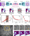
Machine-learned activity field, $\alpha \left(\mathbf{r},t\right)$, in simulations and actin–myosin experiments. (A and B) Machine-learning predicted activity on lattice Boltzmann simulations with spatially uniform activity prescribed to vary linearly (A) and sinusoidally (B) in time. (C) Machine-learning predicted activity on simulations where the central square (dashed line) is activated. (D) Machine-learning predicted activity vs. time on actin–myosin experiments where myosin motors are controlled through light-activated gear shifting. The dashed line indicates when light is switched on. (E and F) Direct image (E) and machine-learning predicted spatial activity profile (F) of a selectively illuminated actin nematic with light-activated gear-shifting motors. For E and F the experimental data are the dataset reported in figure 1 of Zhang et al. (27). Data for D are from the current study, following the approach used in ref. . (Scale bars, 20 $\mathrm{\mu }$m.)

Fig. 5.

Neural networks with a residual architecture as surrogate models of time evolution. (A) Schematic for predicting the time evolution of an active nematic. Individual images are first compressed by a convolutional encoder into a feature vector to reduce the data dimension by fivefold. Time evolution is predicted in the feature space using a residual block, which is composed of a direct shortcut (straight arrow) to preserve the memory from the previous frame and a recurrent layer (cyan box with a purple looped arrow) to capture the change between frames. Based upon the sequence of feature vectors for the past, the residual block generates the next feature vector for the future, which is then translated by a convolutional decoder into an output image. The output is sharpened by first using relaxational dynamics to update defect positions and then using the updated defect positions to sharpen the entire director field. This procedure is iterated and the sharpened image is used as the next frame. (B) Pixelwise error rate $1-⟨|{\mathbf{n}}_{\text{ML}}\cdot {\mathbf{n}}_{\text{LB}}|⟩$ of the predictive model versus time, for different groups of activity in lattice Boltzmann simulations. The gray area shows regions beyond the Lyapunov time for the lattice Boltzmann simulations (Materials and Methods). Here ${\tau }_{\text{d}}=\eta /\alpha$, the characteristic defect lifetime. We observe that measuring the Lyapunov time in units of ${\tau }_{\text{d}}$ yields a common value of $t_{\lambda }\sim 3.6{\tau }_{\text{d}}$. (C) Comparison of time-averaged correlation length in machine-learning and lattice Boltzmann simulations. (D) Comparison of average director-field correlation time $t_{\theta }$ in machine-learning and lattice Boltzmann simulations. Here, ${\tau }_{\text{LC}}$ is an activity-independent viscoelastic relaxation timescale defined as ${\tau }_{\text{LC}}=\gamma a^2/K$, where $\gamma$ is the rotational viscosity (51). (E) A defect nucleation event as seen in experiment and as predicted by the machine-learning model trained on microtubule–kinesin experimental data. Machine–learning predictions depict the magnitude of $\sin \left(2\theta \right)$, where $\theta$ is the angle of the director field. The $\frac{+1}{2}$ and $\frac{-1}{2}$ defects are marked as red and blue dots, respectively. (Scale bar, 100 $\mathrm{\mu }$m.)

Fig. 6.

Performance comparison between physics-inspired machine-learning model and lattice Boltzmann simulations with parameters extracted using the multiparameter estimation network. To make a fair comparison as well as mimic the true experimental constraints, both approaches take director fields only as input, with no prior knowledge of the velocity field. We quantify their performance by measuring the pixelwise error rate $1-⟨|{\mathbf{n}}_{\text{prediction}}\cdot {\mathbf{n}}_{\text{ground truth}}|⟩$. (A) Error rates for predicting the simulated nemato-hydrodynamics at different levels of activity. Red curves show results for the machine-learning model, while purple curves show results for velocity-uninformed lattice Boltzmann predictions. The gray area shows regions beyond the Lyapunov time for the lattice Boltzmann simulations (Materials and Methods). (B) Error rates for predicting the evolution of microtubule–kinesin experiments at different ATP concentrations. Here we emphasize that unlike lattice Boltzmann simulations, the machine-learning model does not implement any physical theory. Nevertheless, its performance matches or exceeds that of lattice Boltzmann simulations.

References

1. Mehta P., et al. , A high-bias, low-variance introduction to machine learning for physicists. Phys. Rep. 810, 1–124 (2019). - PMC - PubMed
1. Carleo G., et al. , Machine learning and the physical sciences. Rev. Mod. Phys. 91, 45002 (2019).
1. Lecun Y., Bengio Y., Hinton G., Deep learning. Nature 521, 436–444 (2015). - PubMed
1. Schmidhuber J., Deep learning in neural networks: An overview. Neural Network. 61, 85–117 (2015). - PubMed
1. Schoenholz S., Cubuk E., Sussman D., Kaxiras E., Liu A., A structural approach to relaxation in glassy liquids. Nat. Phys. 12, 469–471 (2016).
Publication types