Data-driven control of complex networks

Abstract

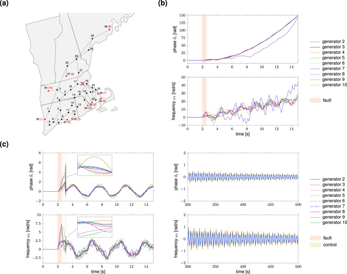
Our ability to manipulate the behavior of complex networks depends on the design of efficient control algorithms and, critically, on the availability of an accurate and tractable model of the network dynamics. While the design of control algorithms for network systems has seen notable advances in the past few years, knowledge of the network dynamics is a ubiquitous assumption that is difficult to satisfy in practice. In this paper we overcome this limitation, and develop a data-driven framework to control a complex network optimally and without any knowledge of the network dynamics. Our optimal controls are constructed using a finite set of data, where the unknown network is stimulated with arbitrary and possibly random inputs. Although our controls are provably correct for networks with linear dynamics, we also characterize their performance against noisy data and in the presence of nonlinear dynamics, as they arise in power grid and brain networks.

Fig. 1. The effect of model uncertainty in the computation of optimal network controls.

Panel (a) shows a schematic of a classic network identification procedure. The reconstructed network is affected by estimation errors δ_ij. The symbol {a_ij} denote the correct network weights, whereas $\left\{{\widehat{a}}_{ij}\right\}$ the (incorrectly) reconstructed ones. Panel (b) illustrates the error in the final (output) state induced by an optimal control design based on the reconstructed network. The symbol y_f denote the desired final state of (a subset of) the network nodes, whereas ${\widehat{\mathbf{y}}}_{\mathrm{f}}$ the one reached by the optimal input u^⋆(t). In panel (c), we consider minimum-energy controls designed from exact and incorrectly reconstructed linear dynamical networks, and compute the resulting error in the final state as the network size n varies. We consider connected Erdös–Rényi networks with edge probability $p_{\mathrm{edge}}=\ln n/n+0.1$, ten randomly selected control nodes, control horizon T = 2n, and a randomly chosen final state ${\mathbf{x}}_{\mathrm{f}}\in {\mathbb{R}}^n$. We assume y_f = x_f, i.e., the nodes that we want to control coincide with all network nodes. To mimic errors in the network reconstruction process, we add to each edge of the network a disturbance modeled as an i.i.d. random variable uniformly distributed in [ − δ, δ], δ > 0. Each curve represents the average of the (norm of the) error in the final state over 100 independent realizations of x_f. To compute minimum-energy control inputs, we use the classic Gramian-based formula and standard LAPACK linear-algebra routines (see “Methods”). Notice that there is a nonzero error in the final state which grows with the size of the network even in the absence of uncertainty (δ = 0). This is due to numerical errors in the computation of the minimum-energy control which are a consequence of the ill-conditioning of the Gramian^,.

Fig. 2. Experimental setup and optimal data-driven network controls.

Panel (a) illustrates the data-collection process. With reference to the ith control experiment, a T-step input sequence ${\mathbf{u}}_{0:T}^{\left(i\right)}$ excites the network dynamics in Eq. (1), and the time samples of the resulting output trajectory ${\mathbf{y}}_{0:T}^{\left(i\right)}$ are recorded. The input trajectory ${\mathbf{u}}_{0:T}^{\left(i\right)}$ may be generated randomly, so that the final output ${\mathbf{y}}_T^{\left(i\right)}$ does not normally coincide with the desired target output y_f. Red nodes denote the control or input nodes (forming matrix B) and the blue nodes denote the measured or output nodes (forming matrix C). Panel (b) shows a realization of the Erdös–Rényi graph model G(n, p_edge) used in our examples, where n is the number of nodes, p_edge is the edge probability. We set the edge probability to $p_{\mathrm{edge}}=\ln n/n+\epsilon$, ε = 0.05, to ensure connectedness with high probability, and normalize the resulting adjacency matrix by $\sqrt{n}$. Panel (c) shows the value of the cost function (left) and the (norm of the) error in the final state (right) for the data-driven input (4) and the model-based control as a function of the number of data points. The symbol y_f denotes the desired final target and ${\widehat{\mathbf{y}}}_{\mathrm{f}}$ the output reached by the (model-based or data-driven) control input. We choose Q = R = I, n = 1000, T = 10, m = 50, and p = 200, and consider Erdös–Rényi networks as in panel (b). For additional details, see “Methods”.

Fig. 3. Performance of minimum-energy data-driven network controls.

Panel (a) shows the value of the cost function (left) and the (norm of the) error in the final state (right) for the minimum-energy data-driven controls (5) and (6), and the model-based one as a function of the data size N. We consider Erdös–Rényi networks as in Fig. 2b with ε = 0.05, and parameters n = 1000, T = 10, m = 50, p = 200. In panels (b–d), we assume C = I and compare the error in the final state generated by the data-driven minimum-energy controls (5) and (6) and model-based expression for a fixed number of control nodes m = 100 and increasing dimension n ∈ [100, 1000]. The model-based control has been computed by first estimating matrices A and B from data according to the subspace-based technique in “Methods”, and then using the model-based control expression. In panel (b), we consider Erdös–Rényi networks with average degree 〈k〉 = 10 (top) and 〈k〉 = 20 (bottom). In panel (c), we consider Barabasi–Albert networks with the initial number of nodes m₀ = 20 and average degree 〈k〉 = 10 (top) and 〈k〉 = 20 (bottom). In panel (d), we consider Watts–Strogatz networks with rewiring probability p_rew = 0.2 and average degree 〈k〉 = 10 (top) and 〈k〉 = 20 (bottom). In all plots, we use a control horizon T = 15 and a number of the data N = mT + 200. To limit the influence of eigenvalues in the computation of optimal controls across different network models, we normalize matrix A by its norm ∥A∥. The curves represent the average of over 100 realizations of networks, data, control nodes, and final states. Panel (e), left, compares the time needed to compute the optimal controls via data-driven and model-based strategies as a function of the network size, for one realization of the Erdös–Rényi model of Fig. 2b and data. Panel (e), right, shows the errors in the final state. We use the following parameters: ε = 0.05, m = ⌊n/100⌋, p = ⌊n/50⌋, T = 50, and N = mT + 100. For additional details, see “Methods”.

Fig. 4. Data-driven control of synchronized patterns in a ring of Kuramoto oscillators.

We consider a ring network of n = 10 Kuramoto oscillators for two different configurations of control nodes (red nodes), namely m = 10 (a) and m = 3 (d). For both configurations, we apply the data-driven control (Eq. (4) of the main text) to steer the phases from the splay state $\left\{{\overline{\theta }}_{1,i}\left(t\right)\right\}$ to the synchronous state (b, e) and from the splay state $\left\{{\overline{\theta }}_{2,i}\left(t\right)\right\}$ to $\left\{{\overline{\theta }}_{1,i}\left(t\right)\right\}$ (c, f). The green region denotes the application of the control. We choose as parameters T = 50 samples of the discretized dynamics (corresponding to a control horizon of 0.5 s), Q = 5I, R = I, and N = 1000 data obtained by perturbing the initial equilibrium with i.i.d. Gaussian inputs with zero mean and standard deviation 0.1.

Fig. 5. Data-driven fault recovery in the New England power-grid network.

Panel (a) depicts the 39-node New England power-grid network (see ref. , Appendix A). The black nodes {1, …, 29} represent load nodes, while the red nodes {30, …, 39} are power generators. The generators are labeled according to the numbers in the red brackets. The red cross denotes the location of the fault. Panel (b) plots the behavior of the phases and frequencies of generators {2, …, 10} after the occurrence of the fault. The onset time of the fault is t = 2 s and the fault duration is 0.5 s (red area in the plots). At time t = 2.5 s the fault is cleared. The phase and frequency of generator 1 (not shown) are fixed to a constant (see “Methods”). The left plots of the panel (c) show the behavior of the phases and frequencies of generators {2, …, 10} after the application of the data-driven control input (4). The duration of the control action is 0.1 s (green area in the plots) which corresponds to a control horizon T = 400 for the discretized network dynamics with sampling period T_s = 2.5 × 10⁻⁴ s. For the computation of the control input, we employ N = 4000 experimental data collected offline by perturbing the state of the generators locally around its steady-state value (see “Methods”). We use weighting matrices R = I and Q = εI, with ε = 0.01. The insets illustrate the behavior of the phases and frequencies during the application of the control. The right plots of the panel (c) show the asymptotic behavior of the phases and frequencies of generators {2, …, 10} after the application of the data-driven control (4).

Fig. 6. Data-driven control of functional brain networks.

Panel (a) provides a schematic of the experimental setup. A set of external stimuli represented by m different task commands induce brain activity. Functional magnetic resonance (fMRI) blood oxygen level-dependent (BOLD) signals are measured and recorded at different times and converted into p time series, one for each brain region. The top and center heatmaps of the panel (b) show the inputs and outputs, respectively, for the first 110 measurements of one subject of the HCP dataset. The inputs are divided into m = 6 channels corresponding to different task conditions, i.e., CUE (a visual cue preceding the occurrence of other task conditions), LF (squeeze left toe), LH (tap left fingers), RF (squeeze right toe), RH (tap right finger), and T (move tongue). As in ref. , each input is a binary 0–1 signal taking the value 1 when the corresponding task condition is issued and 0 otherwise. The outputs represent the BOLD signals of the p = 148 brain regions obtained from and enumerated according to the Destrieux 2009 atlas. The bottom heatmap of the panel (b) displays the simulated outputs obtained by exciting the approximate low-dimensional linear model of ref.  with the input sequence of the top plot. In panel (c), we compare the performance of the data-driven and model-based strategy, assuming that the dynamics obey the above-mentioned approximate linear model. We set the control horizon to T = 100 and generate the data matrices by sliding a time window of size T across the data samples. The target state y_f,i is the eigenvector associated with the i-th eigenvalue of the empirical Gramian matrix ${\widehat{\mathcal{W}}}_T={\widehat{\mathcal{C}}}_T^{\mathsf{T}}{\widehat{\mathcal{C}}}_T$, where ${\widehat{\mathcal{C}}}_T={\mathbf{Y}}_T{\mathbf{U}}_{0:T-1}^{†}$. The left plot shows the error to reach the targets ${\left\{{\mathbf{y}}_{\mathrm{f},i}\right\}}_{i=1}^{20}$ using the data-driven minimum-energy input in Eq. (5) and the model-based one. The right plot shows the norm of the two inputs. The colored bars denote the mean over 100 unrelated subjects and the error bars are the 95% confidence intervals around the mean.

References

1. Levine S, Pastor P, Krizhevsky A, Ibarz J, Quillen D. Learning hand-eye coordination for robotic grasping with deep learning and large-scale data collection. Int. J. Robot. Res. 2018;37:421–436. doi: 10.1177/0278364917710318. - DOI
1. Marx V. Biology: the big challenges of big data. Nature. 2013;498:255–260. doi: 10.1038/498255a. - DOI - PubMed
1. Sejnowski TJ, Churchland PS, Movshon JA. Putting big data to good use in neuroscience. Nat. Neurosci. 2014;17:1440. doi: 10.1038/nn.3839. - DOI - PMC - PubMed
1. Einav L, Levin J. Economics in the age of big data. Science. 2014;346:1243089. doi: 10.1126/science.1243089. - DOI - PubMed
1. Turk-Browne NB. Functional interactions as big data in the human brain. Science. 2013;342:580–584. doi: 10.1126/science.1238409. - DOI - PMC - PubMed
Publication types
LinkOut - more resources