Group testing as a strategy for COVID-19 epidemiological monitoring and community surveillance

Abstract

We propose an analysis and applications of sample pooling to the epidemiologic monitoring of COVID-19. We first introduce a model of the RT-qPCR process used to test for the presence of virus in a sample and construct a statistical model for the viral load in a typical infected individual inspired by large-scale clinical datasets. We present an application of group testing for the prevention of epidemic outbreak in closed connected communities. We then propose a method for the measure of the prevalence in a population taking into account the increased number of false negatives associated with the group testing method.

Fig 1

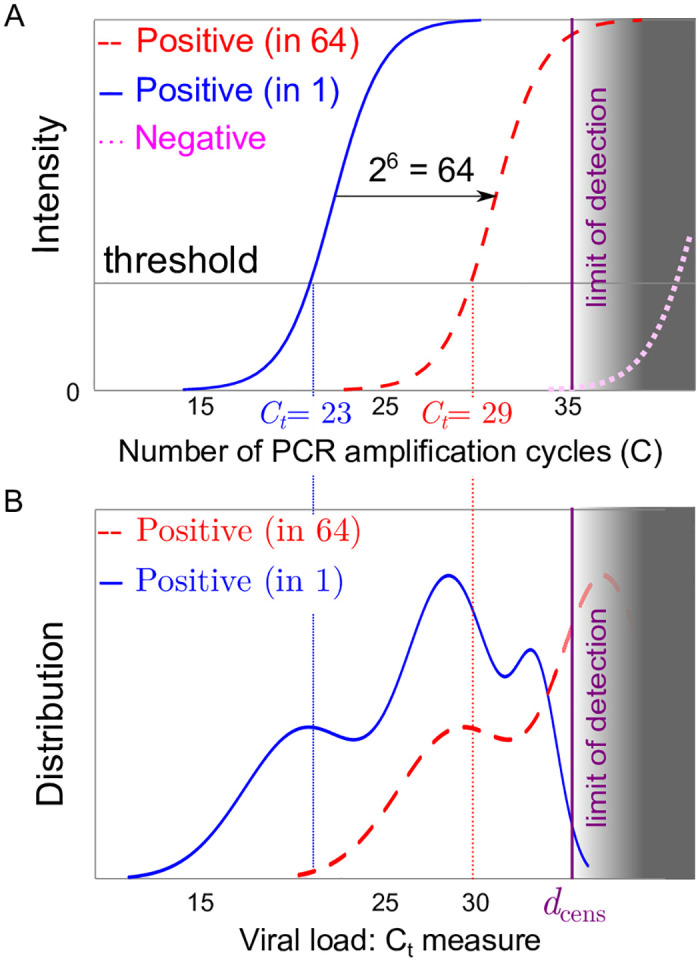
(A) Sketch of an RT-qPCR fluorescence intensity signal for a positive patient without pooling (solid red line) a single positive patient in a pool of 64 patients (dashed red curve) and for a negative sample representing the response of an artefact (dotted magenta curve); as pooling dilutes the initial concentration, the pooled response (dashed red curve) is expected to be close to the translation x → x + 6 from that of a single patient (solid red line). (B) Sketch of the distribution of threshold values for RT-qPCR individual tests (solid blue line) or in pools 64 (dashed red curve); part of the distribution crosses the limit of detection of the test (figured as the grey area) at the detection threshold d_cens.

Fig 2

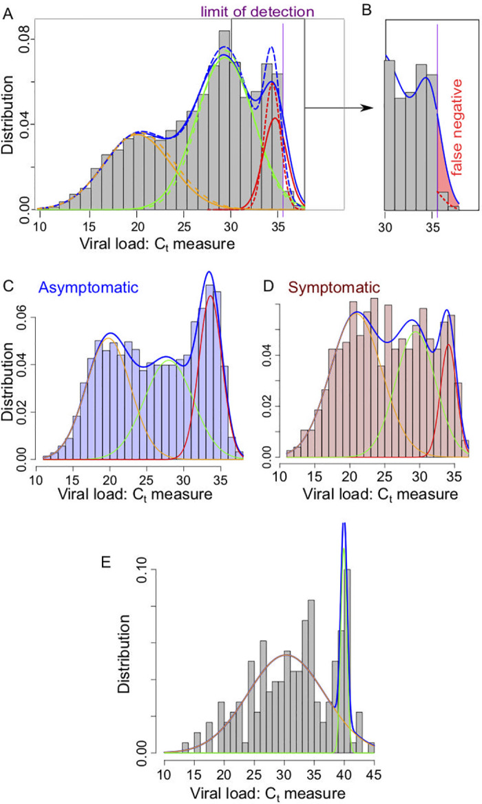
(A) Representation of the density for the classical mixing Gaussian model (dashed lines) and the partially censored model (solid lines) each composed as a sum of 3 components for the Gaussian model (orange/green/red dashed lines) and the partially censored model (orange/green/red solid lines); (purple vertical line) location of the threshold d_att ≈ 35.6. Data based on the histogram presented in [56]. (B) Focus on the false negative region, with the estimated false negative probability in the partially censored model (solid line) due to the defect of detection above the threshold d_att (red color filled area). (C) Mixing Gaussian model on the ImpactSaliva dataset presented in [54]. (D-E) Mixing Gaussian model on the ImpactSaliva dataset presented in [55] for (D) asymptomatic and (E) symptomatic individuals at the moment of the test. Raw data available in S1 Data.

Fig 3

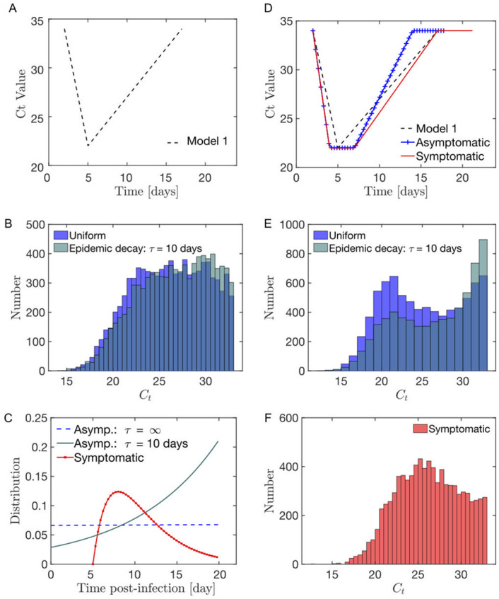
(A) Model 1 for the evolution of the viral load post-infection. (B) Modelled distribution in the infection age at the moment of the test for (red) symptomatic individuals as a Gamma function; (blue-cyan) fully asymptomatic (i.e. throughout the infection) individuals either as (blue) a constant if the new infections rate is a constant with time or (cyan) as an exponential if the rate of new infections decays exponentially with time (characteristic decay time τ = 10 days). (C) In the Model 1 context, the distribution of the viral load in asymptomatic individuals is relatively uniform. (D) Model 2 for the evolution of the viral load post-infection distinguishing between symptomatic and asymptomatic (combining [58] and [59]). Parameters estimate are provided in Table H in S1 Text. (E) In the model 2 context, the distribution of the viral load in asymptomatic individuals shows 2 peaks at high and low viral loads. (F) The distribution of the viral load in symptomatic individuals is less bimodal than the observed asymptomatic distribution.

Fig 4

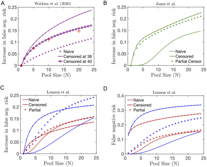
(A-C) Relative increase in the false negative risk $(1-\Phi \left(d_{\text{cens}}^{\left(N\right)}\right))/(1-\Phi \left(d_{\text{cens}}^{\left(1\right)}\right))$ in pools of size N including a single infected individual whose viral distribution is estimated using the naive (solid line), partially censored (circle) or fully censored (crossed line) fitting method of the following datasets from (A) Watkins et al. [54], (B) Jones et al. [56] and (B) Lennon et al. [55]. In (A), we superpose the clinical estimation of the risk of false negative provided in [54] (red crosses). Here, in contrast to [26], we do not change the threshold level of positivity compared to the individual test.

Fig 5

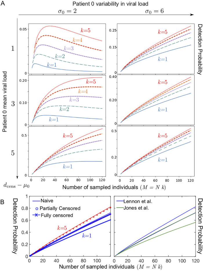
Detection probability within a community of 120 as a function of the total number of sampled individuals M = k × N, where k is the total number of tests used and N the number of samples pooled together in a test (A) Case of a single patient 0 with low viral load; k = 5 (red dotted line); k = 4 (orange line with arrow), k = 3 (purple line with circles); k = 2 (dashed green line); k = 1 (solid blue line) for several values in the parameters describing the viral load of the patient 0 at the onset of contagiosity, expressed in terms of a normal distribution in C_t (the number of RT-qPCR amplification cycles) with a standard deviation σ₀ and a mean μ₀ and a threshold at a value denoted d_cens satisfying: μ₀ = d_cens − 1 (top row), modelling a patient 0 with a very low viral concentration, μ₀ = d_cens − 3 (middle row), μ₀ = d_cens − 5 (bottom row); σ₀ = 2 (left column); σ₀ = 6 (right column). (B) Case of a single patient 0 with a viral load distributed datasets(left) for the three fitting methods used to describe the asymptomatic dataset corresponding to Lennon et al. [55], for k = 1 (blue) and k = 5 (red)and (right) comparing the datasets of Lennon et al. [55] and Jones et al. [56] for the naive fitting method (upper curve k = 5, lower curve k = 1).

Fig 6

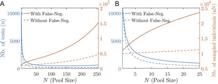
(A,B) Total number of tests (red) and total number of sampled individuals (blue) in order to estimate a prevalence of p = 1% with a ±0.2% precision with 95% confidence interval as a function of the pool size N for the perfect case (dashed lines) with no false negative versus the case with false negatives (solid lines) estimated according to the Lennon et al. asymptomatic dataset [55]. In (A) N ranges from 0 to 25; in (B) N ranges from 0 to 128. The optimal pool size $N_{\text{opt}}^{\text{(perf)}}$ is beyond the N-axis limit.

References

-
- World Health Organization. Laboratory testing for 2019 novel coronavirus (2019-nCoV) in suspected human cases. WHO—Interim guidance. 2020;2019(January):1–7.
- Gollier C, Gossner O. Group Testing against Covid-19. Covid Economics. 2020; p. 32–42.
MeSH terms
LinkOut - more resources
Full Text Sources
Other Literature Sources