Application of single-cell transcriptomics to kinetoplastid research

Abstract

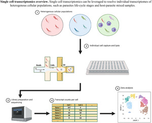
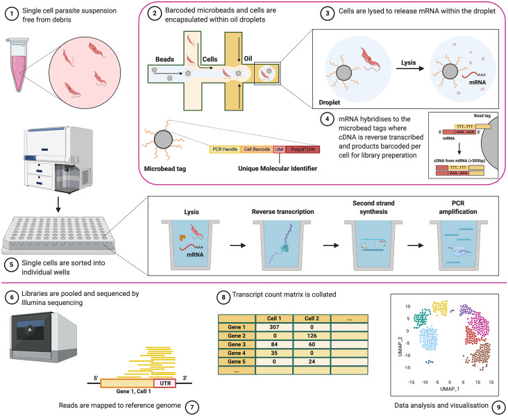
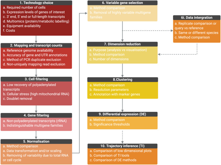
Kinetoplastid parasites are responsible for both human and animal diseases across the globe where they have a great impact on health and economic well-being. Many species and life cycle stages are difficult to study due to limitations in isolation and culture, as well as to their existence as heterogeneous populations in hosts and vectors. Single-cell transcriptomics (scRNA-seq) has the capacity to overcome many of these difficulties, and can be leveraged to disentangle heterogeneous populations, highlight genes crucial for propagation through the life cycle, and enable detailed analysis of host–parasite interactions. Here, we provide a review of studies that have applied scRNA-seq to protozoan parasites so far. In addition, we provide an overview of sample preparation and technology choice considerations when planning scRNA-seq experiments, as well as challenges faced when analysing the large amounts of data generated. Finally, we highlight areas of kinetoplastid research that could benefit from scRNA-seq technologies.

Keywords: bioinformatics; gene expression; kinetoplastid; parasitology; single-cell transcriptomics.

Graphical abstract

Fig. 1.

Overview of the scRNA-seq experimental approach. Single parasites, suspended free from debris and containing ideally >90% viable cells, (1) can be captured individually with barcoded library adaptors and lysis buffer either via droplet-based technology (2) or by sorting into individual plate-wells (5). Cells are then lysed (3) and polyadenylated RNA is reverse transcribed with barcode adaptors into cDNA and amplified (4). The resultant library is then sequenced by next-generation sequencing (6). Reads are mapped to the reference genome (7), and unique reads mapping to each gene are counted to generate raw transcript counts per gene, per cell (8). Quality control filtering, pre-processing and final analysis can then be performed (9). See Fig. 4 for an analysis overview. Note, Seq-well, which uses microarrays to capture cells, is not described in this figure but has been used to study T. gondii parasites (Waldman et al., 2020) (created with BioRender.com).

Fig. 2.

Comparison of methanol fixed and live T. brucei Chromium scRNA-seq data. Methanol fixed (20,000 cells; 1,804 recovered) and live (15,000 cells; 6,938 recovered) T. brucei bloodstream form parasites were previously subjected to Chromium scRNA-seq to a depth of ~30,000 reads per cell (Briggs et al., 2020). (A) UMI (unique molecular identifier;x-axis) and gene (y-axis) per cell counts for methanol fixed (above, red) and live (below, blue) cells. Each point is one cell. The red dashed line indicates the QC threshold used for filtering each sample. (B) As in a, where the percentage of transcripts aligning to the maxi circle kDNA sequence is used as a QC threshold (y-axis). (C) As in a, with a percentage of transcripts aligning to rRNA genes used as a QC threshold (y-axis). (D) UMAPs of each sample (methanol-fixed above, live below), generated as described previously (Briggs et al., 2020) using an identifical method and parameters, with the expections of the QC thresholds indicated in a, b and c. Each data point is one cell coloured by the cluster identity, where each cluster is a group of cells with similar transcriptomic profiles. Colours are not transferred between plots. (E) UMAP plots of cells coloured by expression of one slender marker gene (GAPDH; Tb927.6.4280) and one stumpy marker gene (PAD2; Tb927.7.5940). The scale shows the raw transcript count per cell.

Fig. 3.

Evaluation of sequencing depth impact on cluster identification and differential gene expression analysis. T. brucei bloodstream form (Briggs et al., 2020) cells were previous subjected to Chromium scRNA-seq (Briggs et al., 2020) to a depth of 52,971 mean reads per cell. (A) Sequencing saturation [1−(number of unique reads/number of total mapped reads)] as calculated by cell ranger (10x Genomics, 2020a) for between 5,000 and 52,971 mean reads per cell. The dashed line is equal to 0.9 (90%) sequence saturation. (B) Median genes per cell for total sequencing (52,971 mean reads per cell) and four downsampled data sets. The shaded area shows standard deviation (SD.) from the mean for all cells after QC filtering to remove cells with <500 unique transcripts. (C) The median number of unique transcripts (UMIs) per cell for each data set, shaded area shows SD (D) Number of differentially expressed (DE) genes identified between clusters shown in e, using MAST (Finak et al., 2015). (E) UMAP plots of each data set. Each data point is one cell coloured by cluster identified with the same parameters (resolution = 0.35). Colours are not transferred between plots. Mean reads per cell for each data set are indicated above in bold. The analysis was performed as described previously (Briggs et al., 2020).

Fig. 4.

Outline of the general scRNA-seq analysis steps and user considerations. General analysis steps are indicate by numbers and points of consideration are listed below each. (1) The choice of technology will depend on the number of cells required, the expression level of genes, whether full-length transcripts are required, equipment availability and costs. Once scRNA-seq is performed, sequencing is mapped, and transcript counts per gene for each cell are calculated (2). Counts data will be affected by the accuracy of the genome, gene and UTR annotations, PCR duplicate removal and non-uniquely mapping reads. Data will then require filtering to remove cells of low quality or doublets (3) and genes for which transcript counts are likely to be inaccurate (4). Once filtered, data will require normalization, the best method for which will be data set-dependant (5). Data can also be scaled to remove variable gene expression due to total RNA per cell differences and cell cycle dependant gene expression variation. For further analysis, only the top variable genes should be selected to avoid introducing noise (6). Genes from multiple selection methods should be considered and some genes may require removal from variable gene lists, such as VSGs, if not under investigation. (6i) Replicate samples can be integrated, or query cells can be mapped to a control data set or cell ‘atlas’ of the same or different species. Methods should be compared and will depend on aims. As it is not possible to work in high-dimensional space, data should then be reduced (7) and the appropriate number of dimensions to include should be tested. The type of dimensional reduction performed will depend on aims (analysis or visualization) (8). Cells can be clustered by gene expression using reduced data and labelled by investigating the expression of marker genes. Cluster numbers will be dependent on parameters such as resolution. Differential expression (DE) analysis can be performed between clusters or between conditions if data is integrated (9). Tools are still under development to improve power and false discovery rates, and so methods should be compared. If investigating a biological progression between cellular states, trajectory inference (TI) can be performed (10). Over 70 tools exist and performance depends on the topology of the data in low-dimensional plots. Results should be compared and DE across trajectories investigated. (Created with BioRender.com)

References

1. 10x Genomics (2020a) Cell ranger – Software overview. Available at: https://support.10xgenomics.com/single-cell-gene-expression/software/ove... (Accessed: 15 December 2020).
1. 10x Genomics (2020b) Chromium Next GEM Single Cell 5′ v2. Available at: https://support.10xgenomics.com/single-cell-vdj/library-prep/doc/technic... (Accessed: 15 December 2020).
1. Alfituri OA, Quintana JF, MacLeod A, Garside P, Benson RA, Brewer JM, Mabbott NA, Morrison LJ and Capewell P (2020) To the skin and beyond: the immune response to African trypanosomes as they enter and exit the vertebrate host. Frontiers in Immunology 11, e1250. doi: 10.3389/fimmu.2020.01250 - DOI - PMC - PubMed
1. Andreatta M and Carmona SJ (2020) STACAS: sub-type anchor correction for alignment in Seurat to integrate single-cell RNA-seq data. Bioinformatics 1, 3. doi: 10.1093/bioinformatics/btaa755 - DOI - PMC - PubMed
1. Angerer P, Haghverdi L, Büttner M, Theis FJ, Marr C and Buettner F (2016) Destiny: diffusion maps for large-scale single-cell data in R. Bioinformatics 32, 1241–1243. doi: 10.1093/bioinformatics/btv715 - DOI - PubMed
Publication types