Modeling and Synthesis of Breast Cancer Optical Property Signatures With Generative Models

Abstract

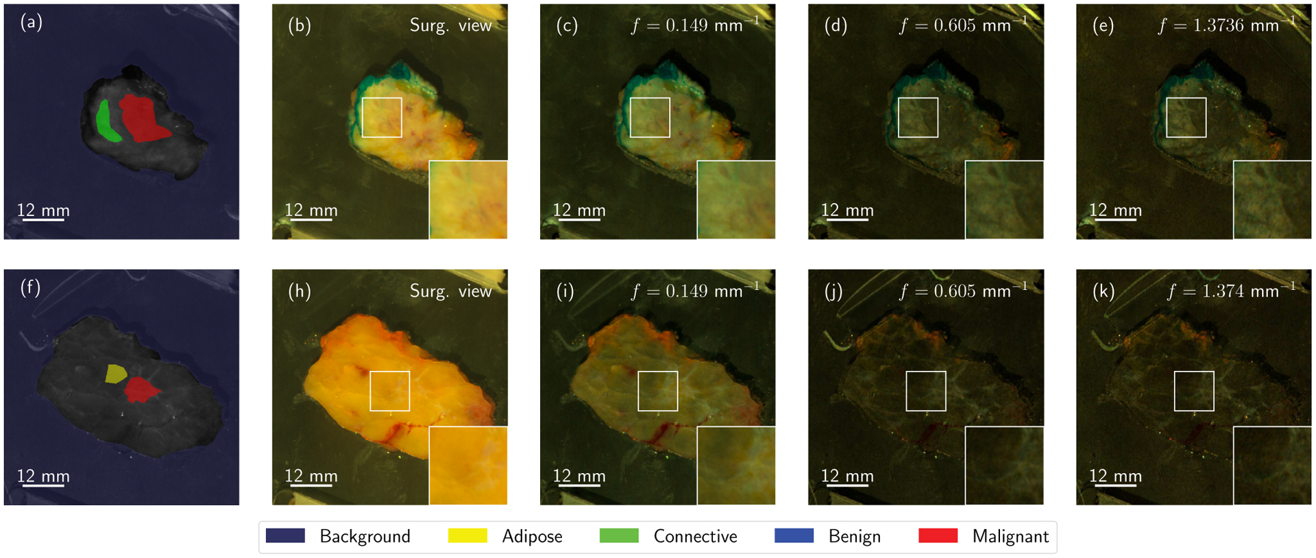
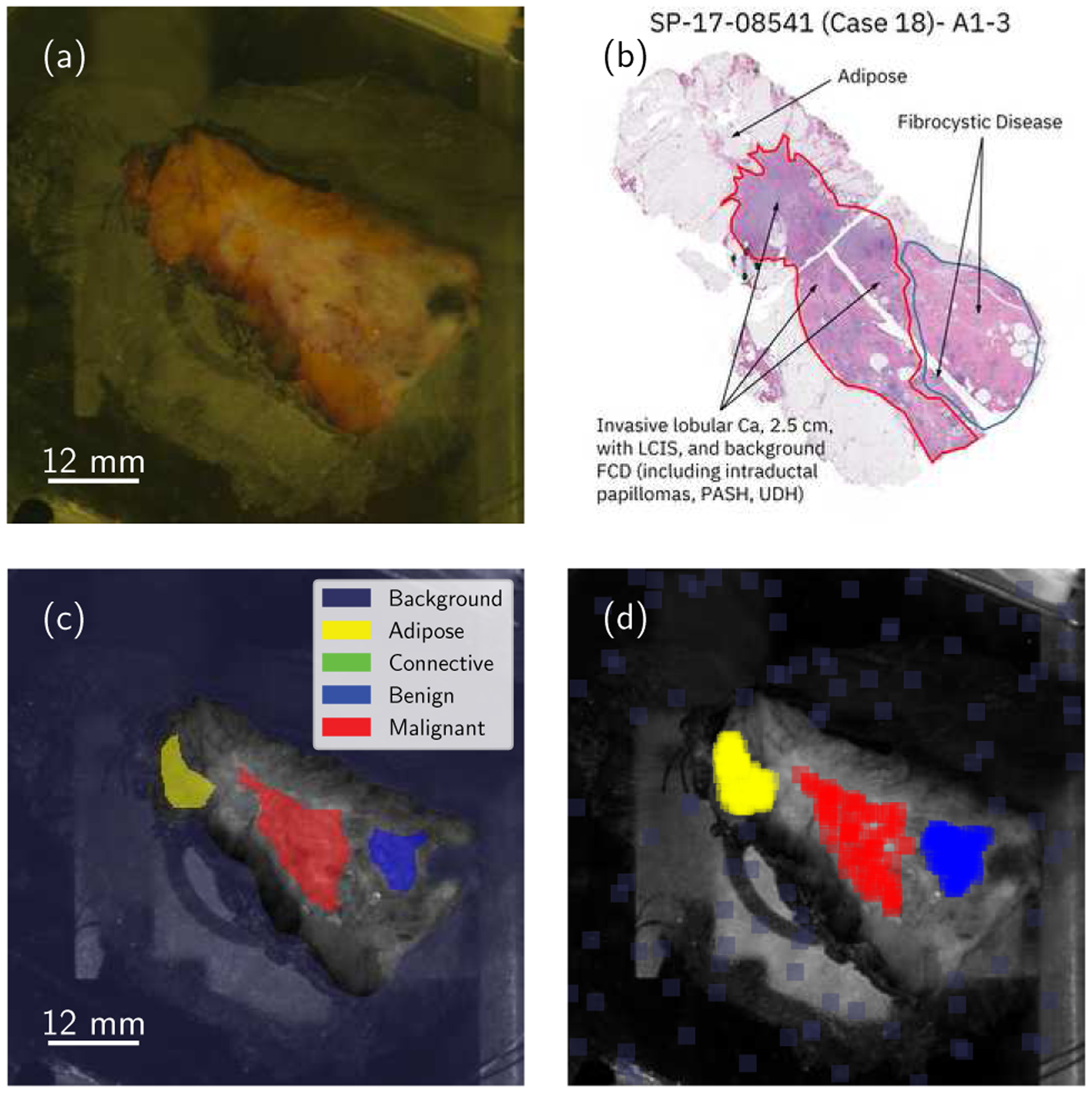
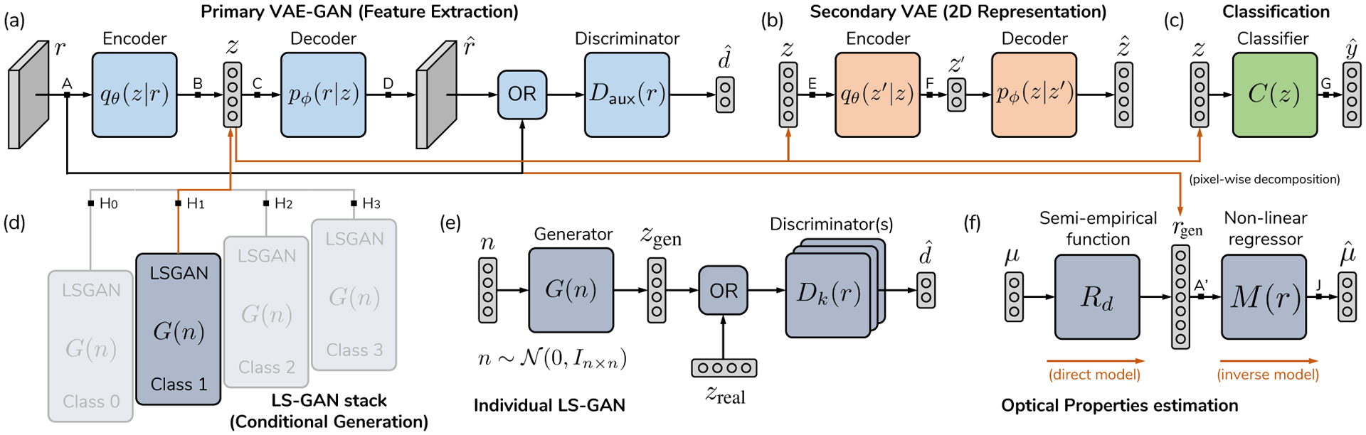
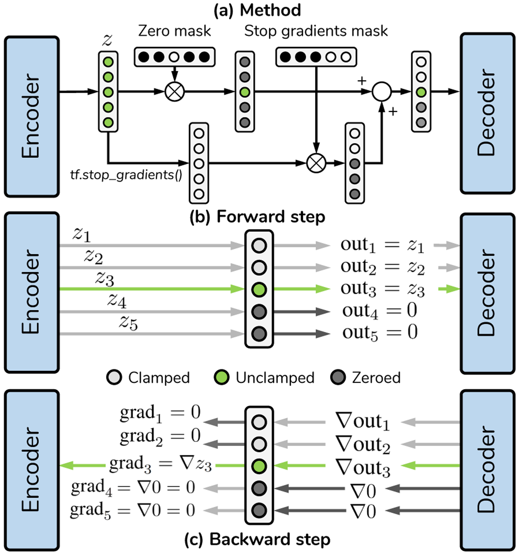
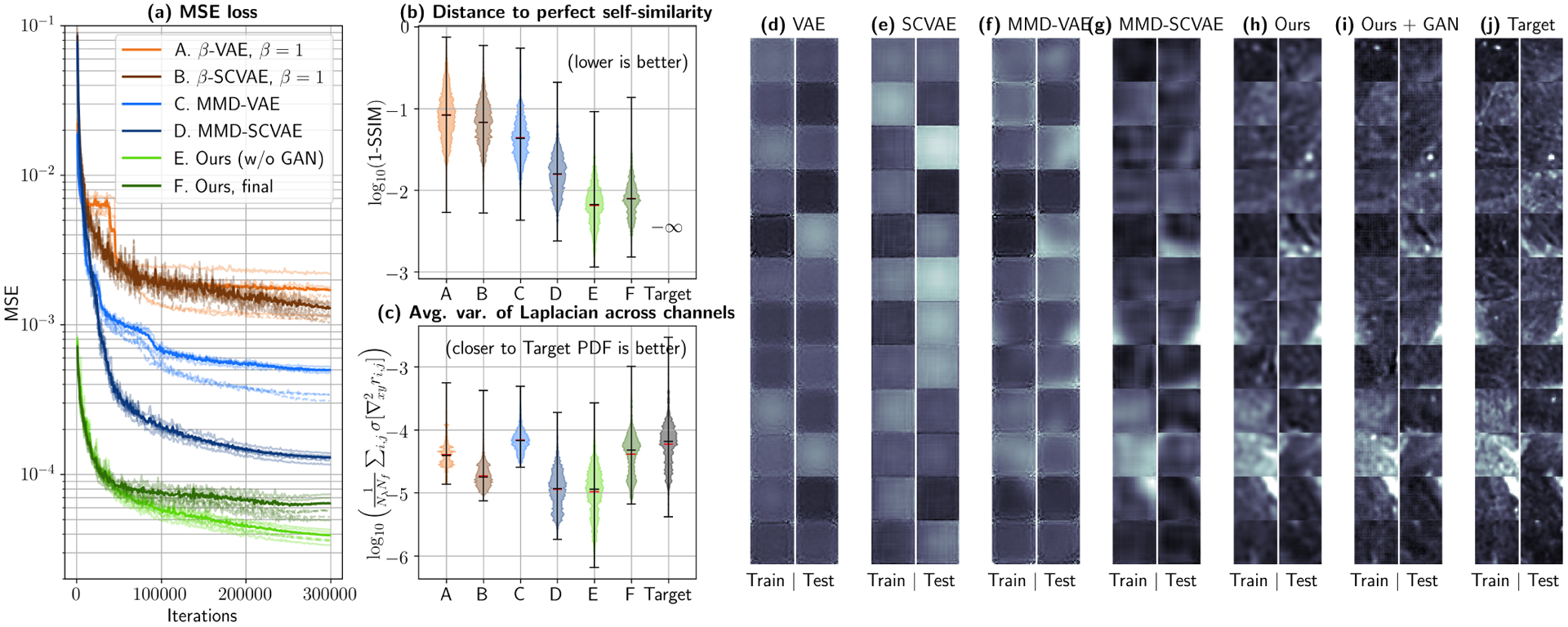
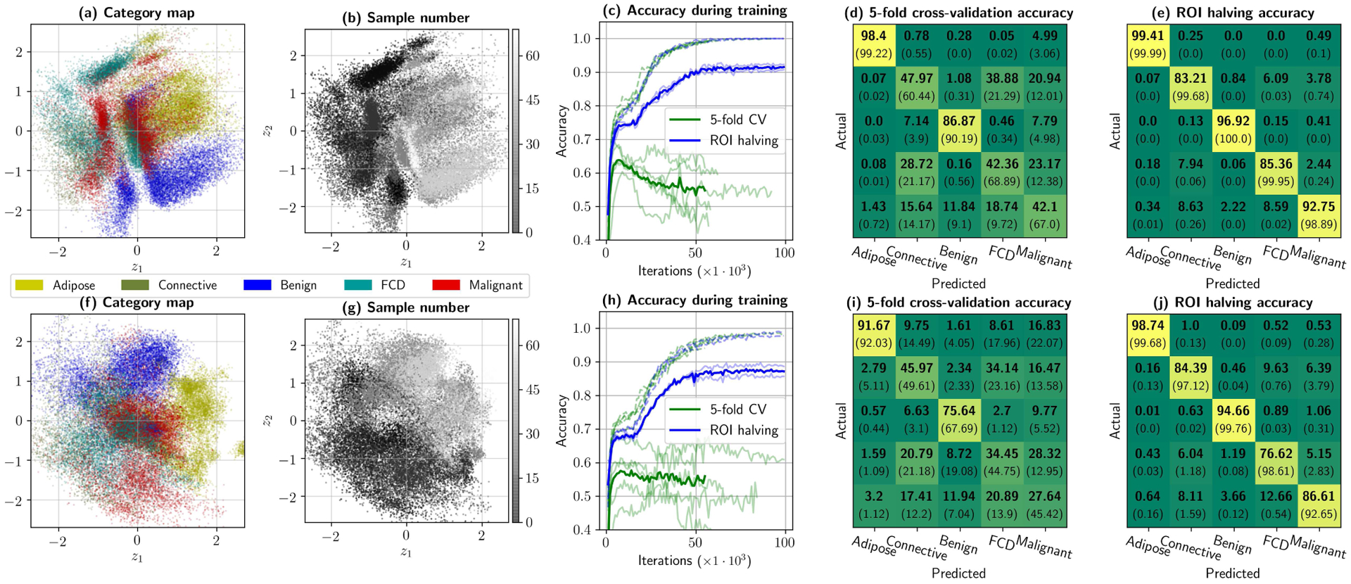
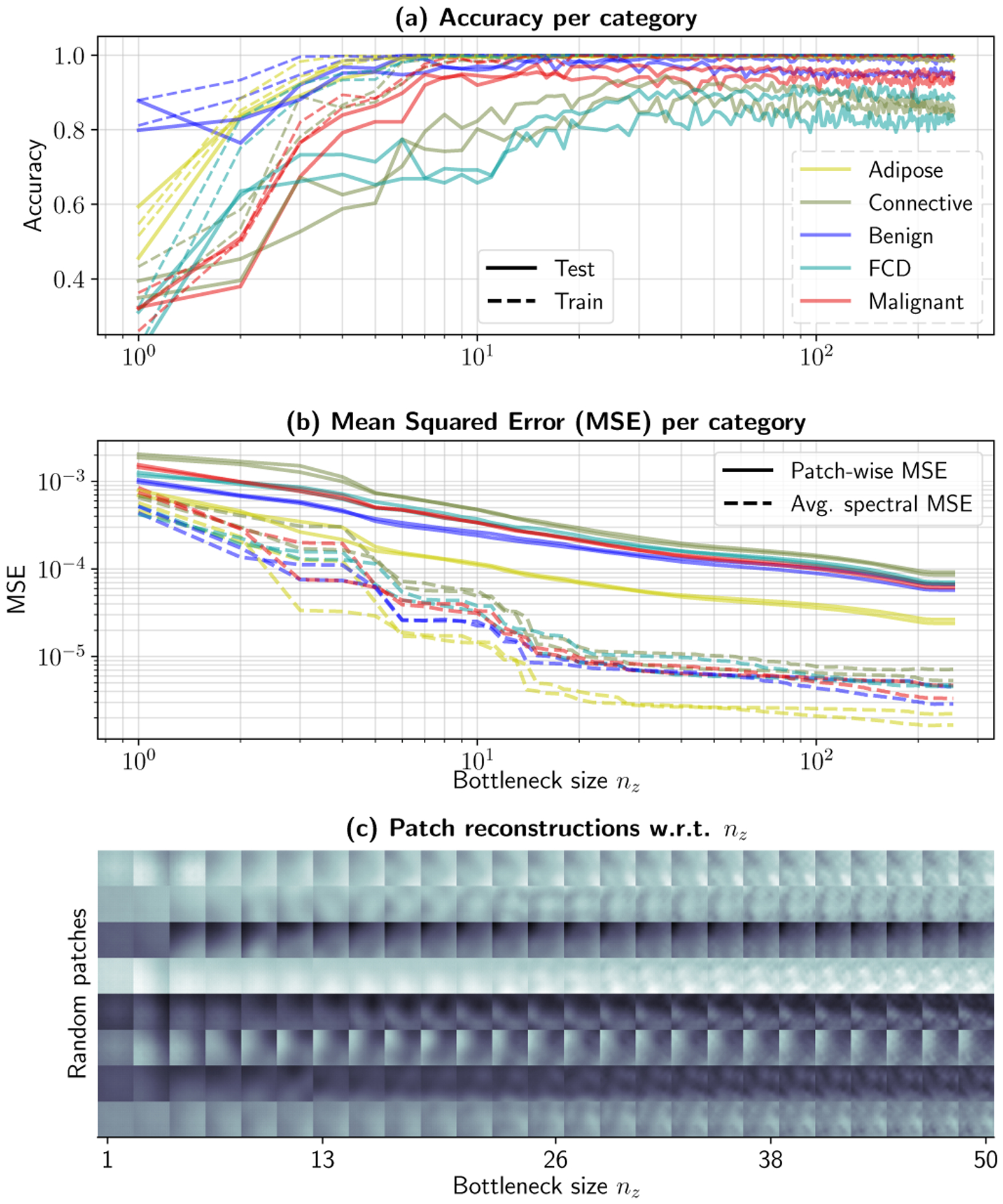
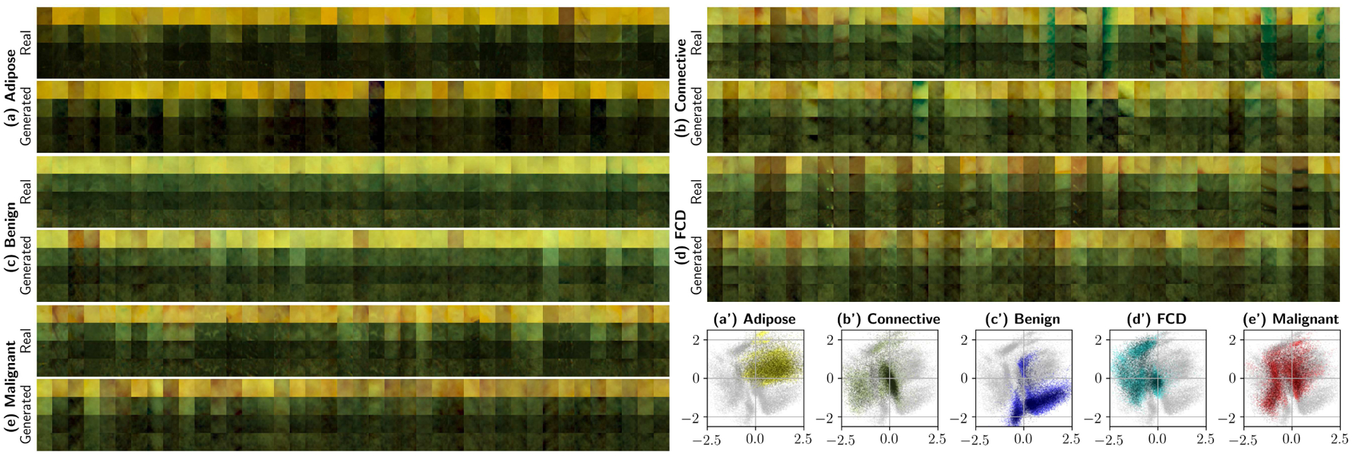
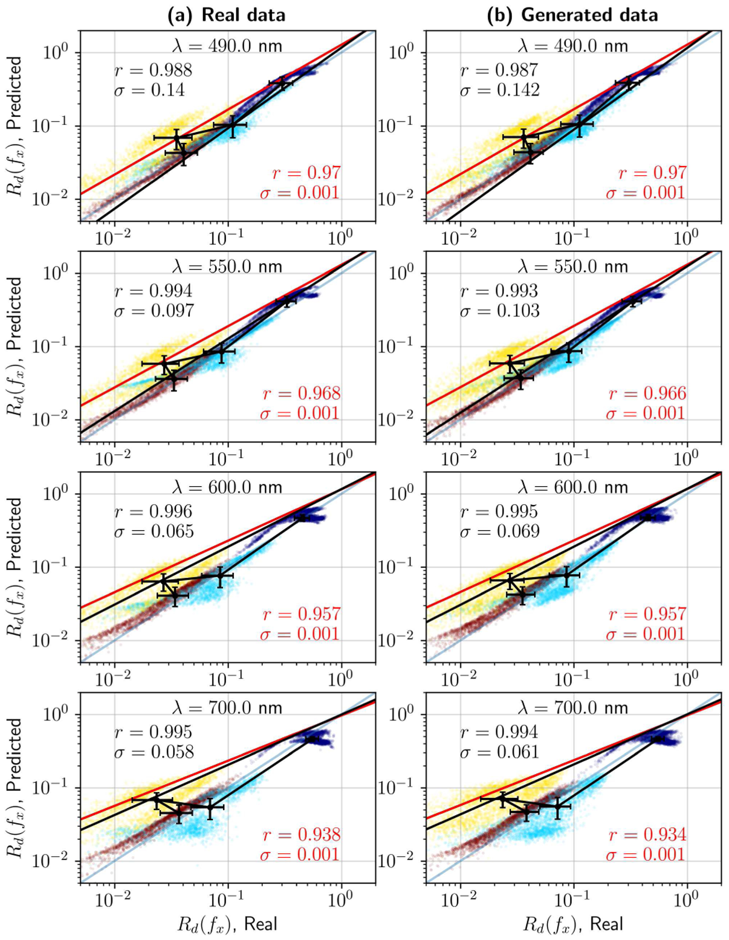
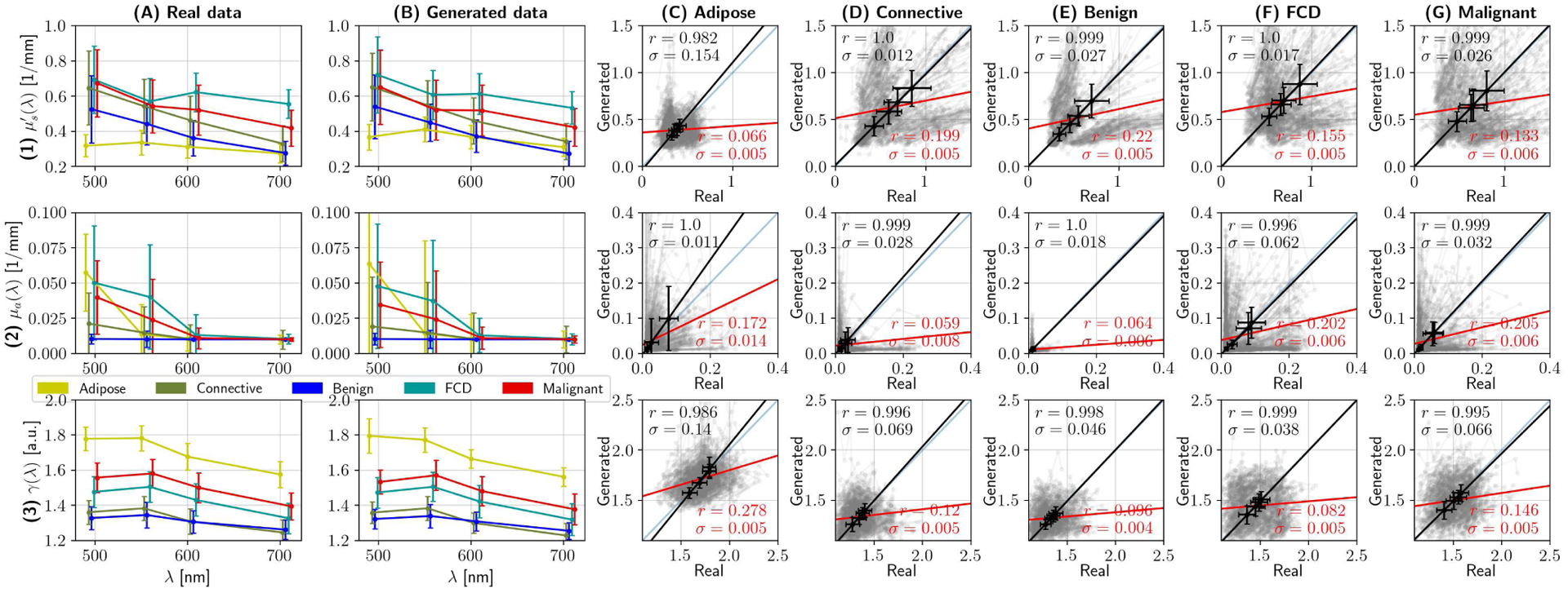
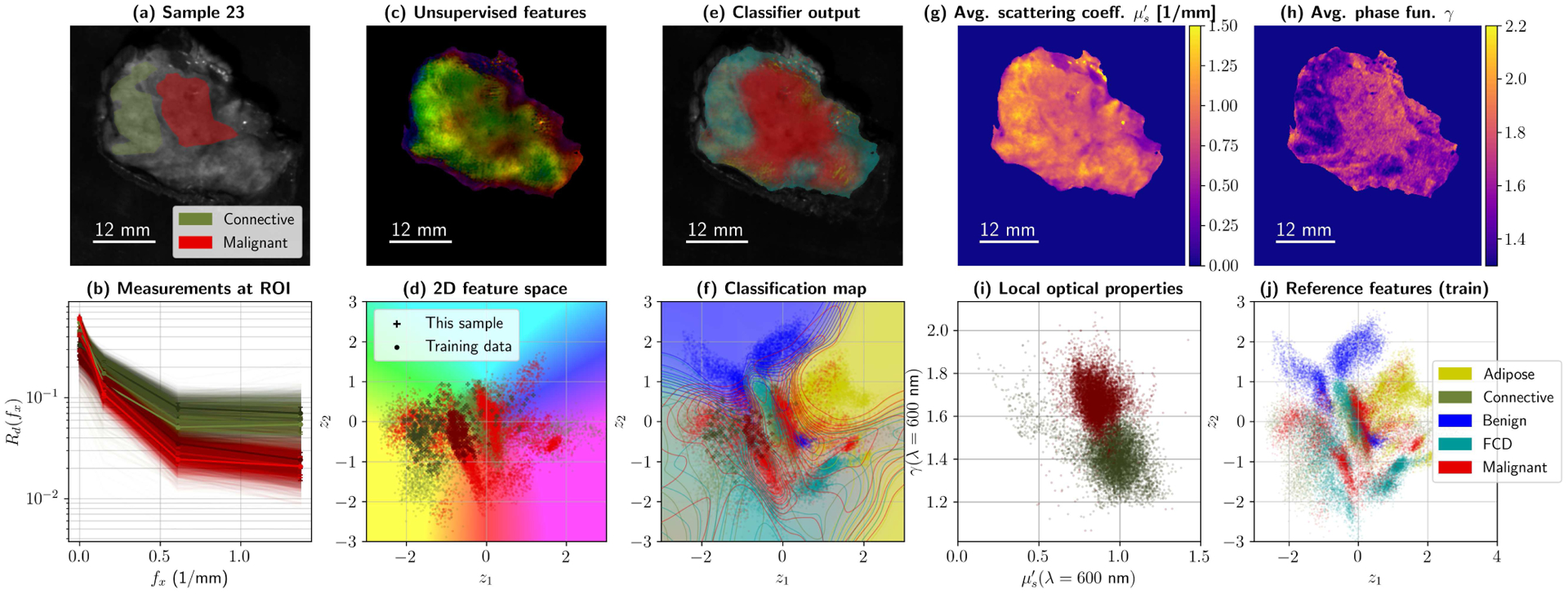
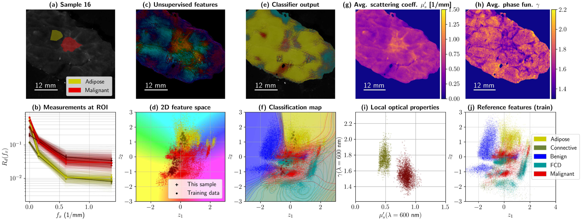
Is it possible to find deterministic relationships between optical measurements and pathophysiology in an unsupervised manner and based on data alone? Optical property quantification is a rapidly growing biomedical imaging technique for characterizing biological tissues that shows promise in a range of clinical applications, such as intraoperative breast-conserving surgery margin assessment. However, translating tissue optical properties to clinical pathology information is still a cumbersome problem due to, amongst other things, inter- and intrapatient variability, calibration, and ultimately the nonlinear behavior of light in turbid media. These challenges limit the ability of standard statistical methods to generate a simple model of pathology, requiring more advanced algorithms. We present a data-driven, nonlinear model of breast cancer pathology for real-time margin assessment of resected samples using optical properties derived from spatial frequency domain imaging data. A series of deep neural network models are employed to obtain sets of latent embeddings that relate optical data signatures to the underlying tissue pathology in a tractable manner. These self-explanatory models can translate absorption and scattering properties measured from pathology, while also being able to synthesize new data. The method was tested on a total of 70 resected breast tissue samples containing 137 regions of interest, achieving rapid optical property modeling with errors only limited by current semi-empirical models, allowing for mass sample synthesis and providing a systematic understanding of dataset properties, paving the way for deep automated margin assessment algorithms using structured light imaging or, in principle, any other optical imaging technique seeking modeling. Code is available.

Fig. 1.

Two lumpectomy samples from the breast tissue dataset, namely samples 23 (top row) and 16 (bottom row). Structured light imaging reveals hidden textural contrast as a function of spatial frequency. Each of the specimens is accompanied by a set of Regions of Interest with known properties (a, f). Here, color reconstructions of demodulated reflectance data for f = 0.0 (b, h), f = 0.15 (c, i), f = 0.61 (d, j), and f = 1.37 mm⁻¹ (e, k) are shown to present how textural properties evolve as a function of the spatial frequency of the projected patterns. Best viewed in color.

Fig. 2.

General summary of the complete data extraction protocol. Each specimen is visually inspected (a) and co-registered with H&E stain histology data (b). This analysis results in conservative, manually-generated Regions of Interest (c) which are then uniformly sampled and filtered depending on additional requirements (d). Best viewed in color.

Fig. 3.

Network setup for the four domain problem. (a) Reflectance data r is introduced into a primary autoencoder (i.e. $r\to z\to \widehat{r}$), generating a low-dimensional translation of spectral and spatial data. (b) A secondary autoencoder $z\to z^{\prime }\to \widehat{z}$ transforms this first domain into a two-dimensional domain z′, where the dataset can be represented. The same codeword z can be used for classification (c). Conditional sample generation is achieved with a set of small multilayer perceptron Least-Squares GANs (d), with multiple decoders to avoid mode collapse (e). Optical properties estimation is achieved via an MLP non-linear regressor, which is trained with domain randomization, using spectra generated by giving random OP values to a deterministic semi-empirical function (f). The following paths represent each of the objectives in Fig. 1, as follows: $\overline{AB}$ (Feature Extraction), $\overline{\mathit{\text{ABEF}}}$ (Visualization), $\overline{\mathit{\text{ABG}}}$ (Classification), $\overline{H_0/\dots /H_{n}CD}$ (Generation), $\overline{A{A}^{\prime }J}$ (pixel-wise OP estimation). Black arrows are real connections in the graph, while orange connections represent copying operations.

Fig. 4.

Bottleneck clamping for dimensionality reduction. Schematic analogous to [51] but for all coordinates in a bottleneck. (a) Process for generating words of length 3 (i.e. training the third unit in z) in a primary bottleneck with n_z = 5. (b) Forward step, showcasing which values are transmitted to the decoder. Units past the third one are zeroed out. (b) Gradient backpropagation of the given keyword. The gradient is cut for all coordinates except the one under training, thus in this step the encoder must modify the third coordinate to improve the reconstruction error given previous unit values. Each unit is trained stochastically within a given minibatch. After training, all units in the bottleneck are left unclamped.

Fig. 5.

Autoencoder comparison via 3-fold cross-validation. (a) Mean Squared Error (MSE) for all the tested architectures. Transparent dashed curves depict training errors, while continuous curves correspond to test errors for each fold. The average test error is shown as a thicker, non-transparent line for each network. Architecture E (MMD-SCVAE with fully connected connections at encoder and decoder, Gradually Upscaling Network and auxiliary fully connected feature maps) achieves the lowest average test MSE in the least amount of iterations. (b) This can also observed by evaluating the distance to a perfect test SSIM (1.0), where architectures E and F show up to an order-of-magnitude improvement in self-similarity when compared to controls. (c) However, most architectures still return blurred reconstructed patches, which can be quantified by the average variance of the Laplacian across channels. By using an auxiliary GAN Discriminator (Architecture F), high frequency components can be better recovered, which translates in a variance histogram that better follows the true distribution. Reconstructions returned by each of the proposed architectures can be qualitatively observed in (d)–(i) and compared with the true data (j). Reflectance values are shown in the range [0.0, 0.04] at spatial frequency f_x = 0.61 mm⁻¹ and wavelength λ = 500 nm.

Fig. 6.

Initial dataset considerations provided by the neural framework. Top row shows (a) the 31 × 31-pixel patch dataset projected into 2D, color-coded by tissue supercategory, (b) the same plot but color-coded by sample number of origin, (c) classifier accuracies observed during training for 1000 random samples of the training and test sets in 5-fold cross-validation and ROI halving experiments. Finally, the confusion matrices in (d) and (e) provide the best test (in bold) and training (between parentheses) accuracies per category, for 5-fold cross-validation and ROI halving, respectively. Bottom row –plots (f) through (j)– provides analogous results for pixel-wise analysis. In this dataset, inter-sample variability dominates intra-sample variability by a significant margin, to the point that spectra can be nearly perfectly identified if the training set includes information from its specimen of origin.

Fig. 7.

An ablation test can evaluate the effect of bottleneck size on classification accuracy and reconstruction quality. Experiment results obtained via ROI halving. Subplot (a) shows per-category classification accuracy for training and test sets for both halves, while (b) evaluates the patch-wise MSE and average spectral MSE between original and reconstructed patches. Finally, (c) shows reconstructions for different bottleneck sizes. Bottleneck clamping allows the use of a single autoencoder for this experiment. The rest of the coordinates are set to zero and the reconstruction is extracted at its output. A high-resolution version of (c) is provided in the Supplementary Material.

Fig. 8.

Generating patches at various frequencies with the LS-GAN stack. The following are outputs of the primary autoencoder to synthesized 256-dimensional feature keywords. This experiment uses the complete dataset (80% for training, 20% for validation). Plots (a) through (d) show spectra-to-RGB reconstructions of real and generated patches, where each column displays a patch at the four different spatial frequencies (0.0, 0.15, 0.61, and 1.37 mm⁻¹). Subplots (a’) through (e’) show 5000 artificially generated samples for each supercategory projected onto the 2D space of the secondary bottleneck (shown in Fig. 6.(a)). In these scatter plots, light colored points represent reference training data, and darker points correspond to the synthesized data. These 2D projections qualitatively ensure correct sample generation without significant mode collapse. Best viewed in color.

Fig. 9.

Optical properties estimation with a neural network LUT. Actual vs. predicted reflectance R_d(f_x) on the real dataset (left column) and synthetic data (right column). Average standard errors for the dataset are within 5% – 15%, as is typical in SFDI-based OP extraction. Rows show the actual and predicted reflectances for individual wavelengths. Each plot includes coefficients of determination and standard errors for the complete dataset (in red) and the dataset averages (in black).

Fig. 10.

Quality assessment of synthesized spectra can be done indirectly, by analyzing optical properties. Rows (1), (2) and (3) show results pertaining to reduced scattering coefficient ${\mu }_s^{\prime }$, absorption coefficient μ_a, and phase function parameter γ, respectively. Columns (A) and (B) show the median optical properties per tissue category as error-bar plots, where whiskers represent one standard deviation, of real and synthesized spectra, respectively. Columns (C) through (G) randomly compare optical properties of real data with synthesized equivalents for each of the main tissue supercategories. In this grid, each subplot contains 500 pairs of optical properties from real and synthesized spectra in grey, the identity line y = x –plotted in blue–, and two linear regression tests. The red line and stats (namely, coefficient of determination and standard error) are the result of applying linear regression on the raw data, while the black line, errorbars and corresponding statistics correspond to analyzing average optical properties. The former provides little information due to the multimodal characteristics of the dataset; however, the latter demonstrates that, on average, the optical properties of the real and synthesized datasets match.

Fig. 11.

Summary for Sample 23 during 5-fold cross-validation (High Grade IDC embedded in connective tissue). Subplot (a) shows ROIs and average reflectance; (b) presents 10% of the reflectance data within those ROIs, at all four wavelengths. Processing the data with the primary and secondary autoencoder produces a map with two values per pixel, which was translated to HSV values to create a false color image (c). The corresponding colors for the false color map are shown with the test spectra from (b) –as well as training data for the categories of interest– in subplot (d). The classifier uses the 256-D pixels from the primary AE to produce a diagnostic map (e). Classification boundaries can also be projected onto 2D (f), by color-coding z-space with the classifier $\left(z^{\prime }\to \widehat{z}\to \widehat{y}\right)$. Finally, optical property maps can be plotted, namely reduced scattering ${\mu }_s^{\prime }$ (g) and phase function parameter γ (h). Local differences in OPs can be observed and plotted as usual (i). The complete training set in z-space for this fold is left, for reference, in (j).

Fig. 12.

Summary for Sample 16 during 5-fold cross-validation (High Grade IDC in adipose tissue). Subplot (a) shows ROIs and average reflectance; (b) presents 10% of the reflectance data within those ROIs, at all four wavelengths. Processing the data with the primary and secondary autoencoder produces a map with two values per pixel, which was translated to HSV values to create a false color image (c). The corresponding colors for the false color map are shown with the test spectra from (b) –as well as training data for the categories of interest– in subplot (d). The classifier uses the 256-D pixels from the primary AE to produce a diagnostic map (e). Classification boundaries can also be projected onto 2D (f), by color-coding z-space with the classifier $\left(z^{\prime }\to \widehat{z}\to \widehat{y}\right)$. Finally, optical property maps can be plotted, namely reduced scattering ${\mu }_s^{\prime }$ (g) and phase function parameter γ (h). Local differences in OPs can be observed and plotted as usual (i). The complete training set in z-space for this fold is left, for reference, in (j).

References

1. Veronesi U, Cascinelli N, Mariani L, Greco M, Saccozzi R, Luini A et al., “Twenty-year follow-up of a randomized study comparing breast conserving surgery with radical mastectomy for early breast cancer,” N Engl J Med, vol. 347, no. 16, pp. 1227–1232, 2002. - PubMed
1. de Boniface J, Frisell J, Bergkvist L, and Andersson Y, “Breast-conserving surgery followed by whole-breast irradiation offers survival benefits over mastectomy without irradiation,” Br J Surg, vol. 105, no. 12, pp. 1607–1614, 2018. - PMC - PubMed
1. Pleijhuis RG, Graafland M, de Vries J, Bart J, de Jong JS, and van Dam GM, “Obtaining adequate surgical margins in breast-conserving therapy for patients with early-stage breast cancer: current modalities and future directions,” Ann Surg Oncol, vol. 16, no. 10, pp. 2717–2730, 2009. - PMC - PubMed
1. Lovrics PJ, Cornacchi SD, Farrokyar F, Garnett A, Chen V, Franic S et al., “Technical factors, surgeon case volume and positive margin rates after breast conservation surgery for early-stage breast cancer,” Can J. Surg, vol. 53, no. 5, pp. 305–312, 2010. - PMC - PubMed
1. Kaczmarski K, Wang P, Gilmore R, Overton HN, Euhus DM, Jacobs LK et al., “Surgeon Re-Excision Rates after Breast-Conserving Surgery: A Measure of Low-Value Care,” J. Am. Coll. Surg, vol. 228, no. 4, pp. 504–512, 2019. - PubMed
Publication types