Deep learning-based point-scanning super-resolution imaging

Abstract

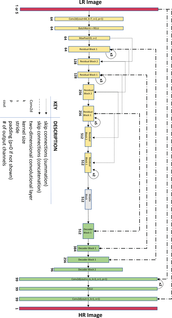
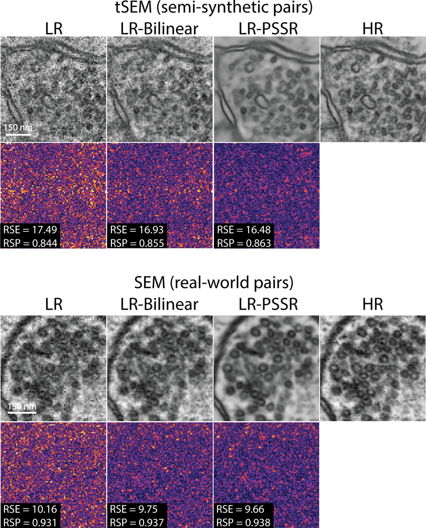
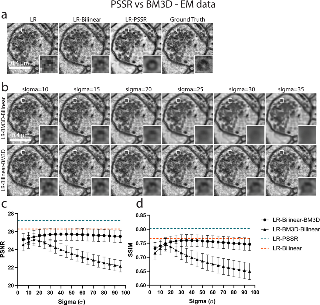
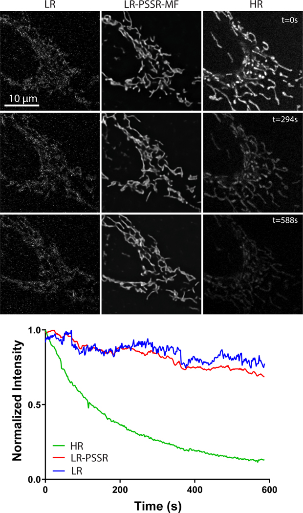
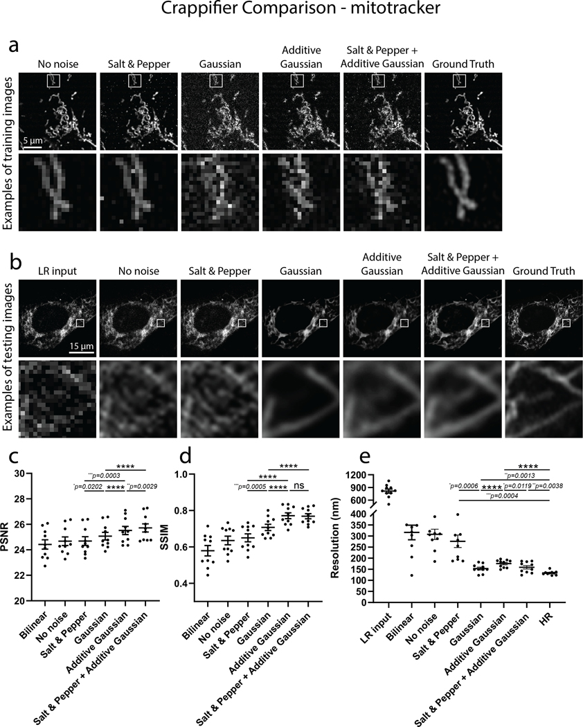
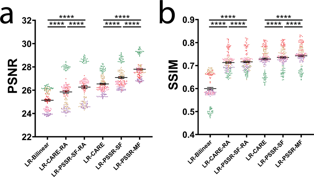
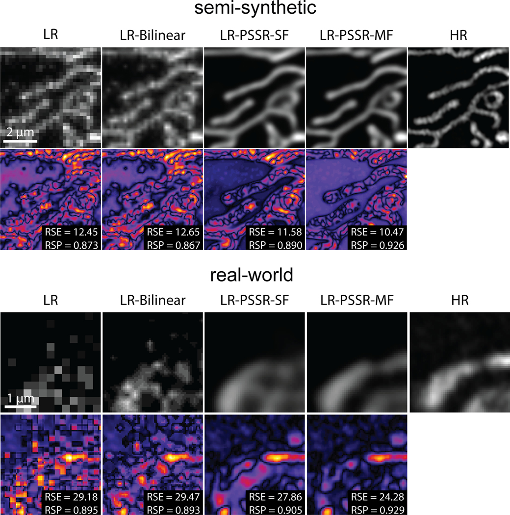
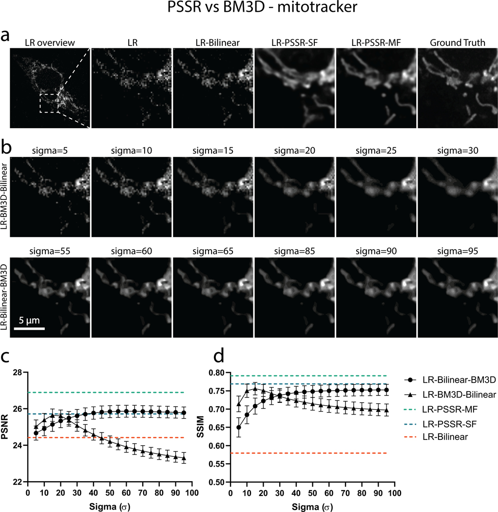
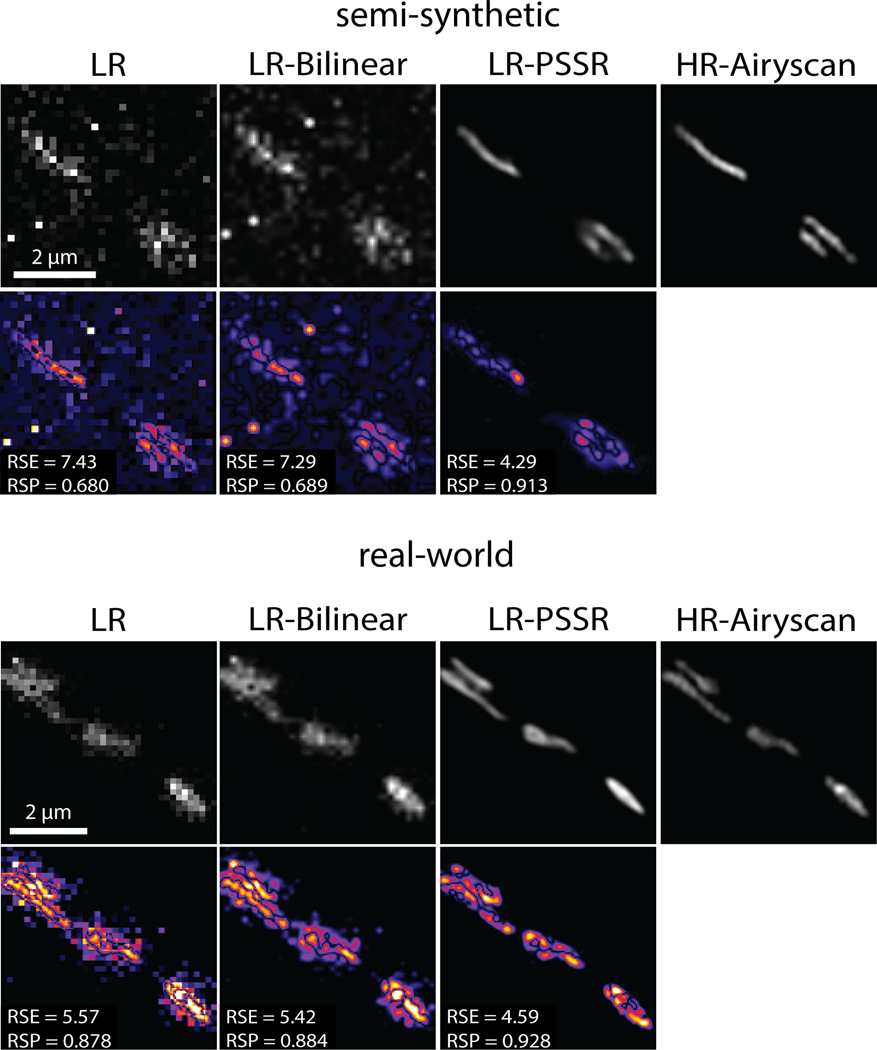
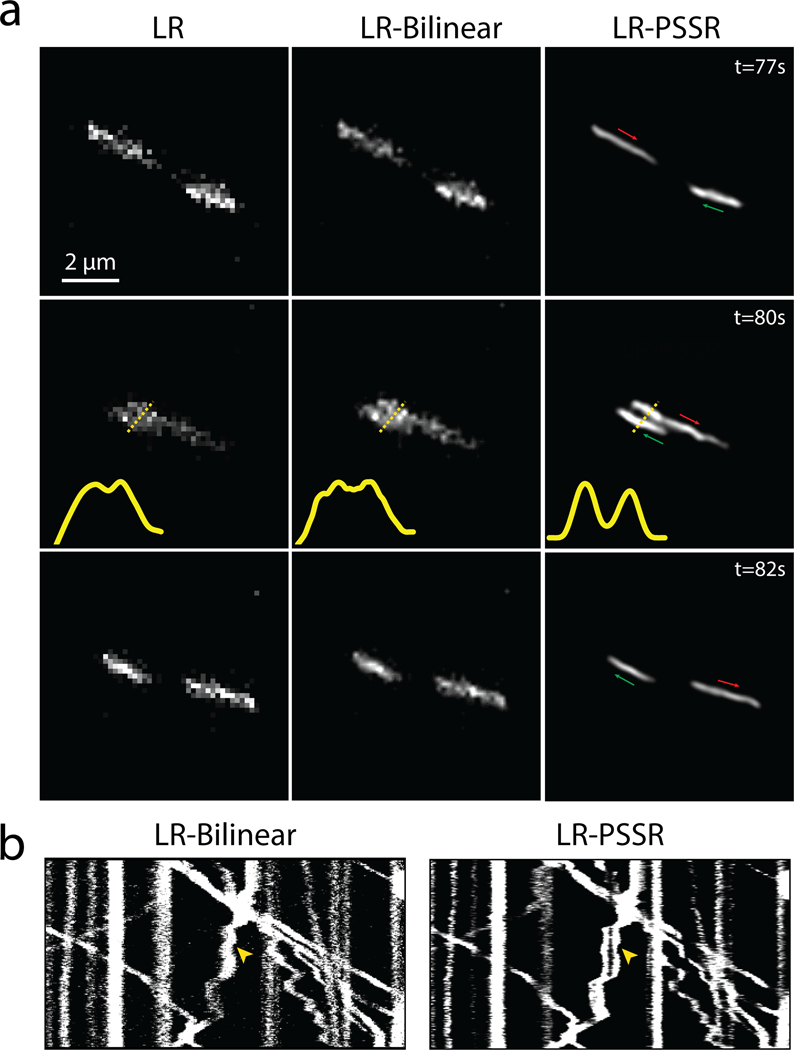
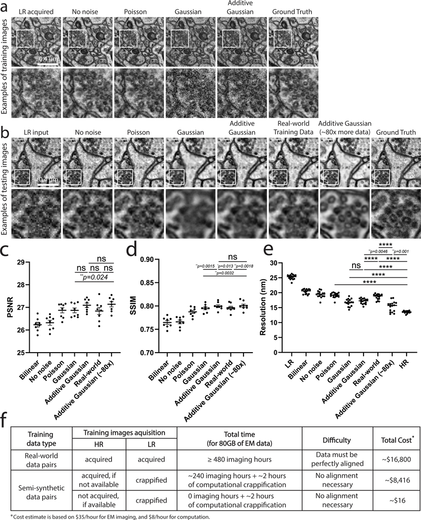
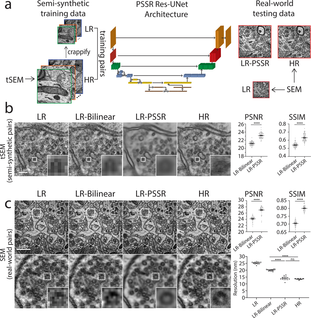
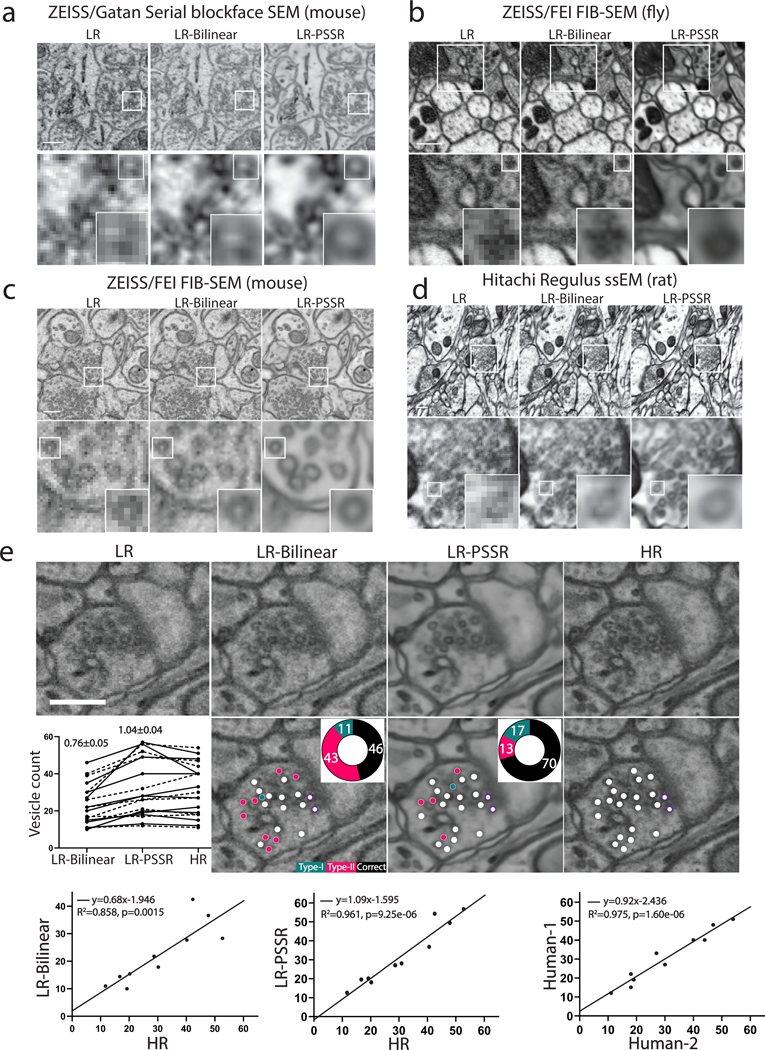
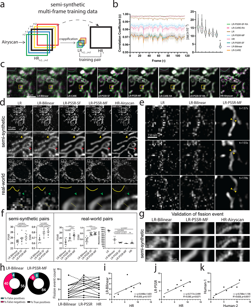
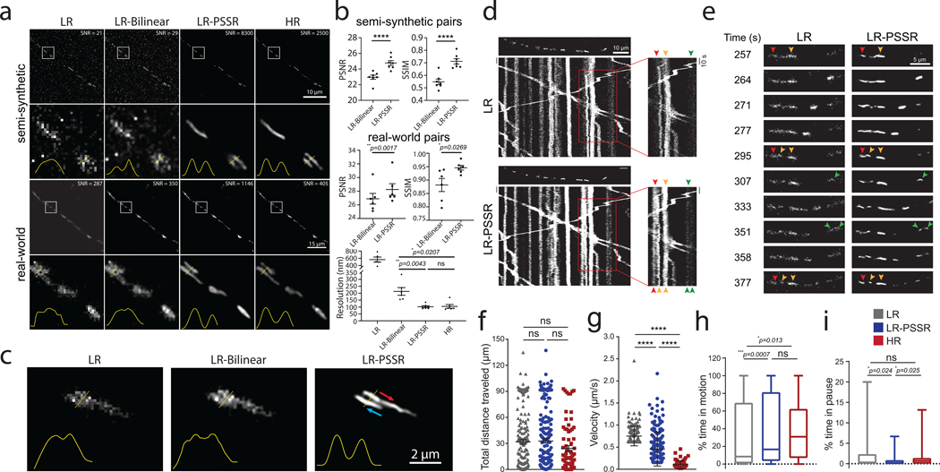
Point-scanning imaging systems are among the most widely used tools for high-resolution cellular and tissue imaging, benefiting from arbitrarily defined pixel sizes. The resolution, speed, sample preservation and signal-to-noise ratio (SNR) of point-scanning systems are difficult to optimize simultaneously. We show these limitations can be mitigated via the use of deep learning-based supersampling of undersampled images acquired on a point-scanning system, which we term point-scanning super-resolution (PSSR) imaging. We designed a 'crappifier' that computationally degrades high SNR, high-pixel resolution ground truth images to simulate low SNR, low-resolution counterparts for training PSSR models that can restore real-world undersampled images. For high spatiotemporal resolution fluorescence time-lapse data, we developed a 'multi-frame' PSSR approach that uses information in adjacent frames to improve model predictions. PSSR facilitates point-scanning image acquisition with otherwise unattainable resolution, speed and sensitivity. All the training data, models and code for PSSR are publicly available at 3DEM.org.

Extended Data Fig. 1. PSSR Neural Network architecture.

Shown is the ResNet-34 based U-Net architecture. Single-frame PSSR (PSSR-SF) and multi-frame PSSR (PSSR-MF) have 1 or 5 input channels, separately.

Extended Data Fig. 2. NanoJ-SQUIRREL error-maps of EM data.

NanoJ-SQUIRREL was used to calculate the resolution scaled error (RSE) and resolution scaled Pearson’s coefficient (RSP) for both semi-synthetic and real-world acquired low (LR), bilinear interpolated (LR-Bilinear), and PSSR (LR-PSSR) images versus ground truth high-resolution (HR) images. For these representative images from Fig. 2, the RSE and RSP images are shown along with the difference images for each output.

Extended Data Fig. 3. Comparison of PSSR vs. BM3D on EM data.

PSSR restoration was compared to the Block-matching and 3D filtering (BM3D) denoising algorithm. BM3D was applied to low-resolution real-world SEM images before (LR-BM3D-Bilinear) and after (LR-Bilinear-BM3D) bilinear upsampling. A wide range of Sigma ($\sigma \in \left(0,\mathrm{ }95\right]$, with step size of 5), the key parameter that defines the assumed zero-mean white Gaussian noise in BM3D method, was thoroughly explored. Images of the same region from the LR input, bilinear upsampled, PSSR restored, and Ground truth is displayed in (a). Results of LR-BM3D-Bilinear (b, top row) and LR-Bilinear-BM3D (b, bottom row) with sigma ranging from [10, 15, … , 35] are shown. PSNR and SSIM results of LR-BM3D-Bilinear and LR-Bilinear-BM3D across the explored range of sigma are plotted in (c) and (d). Metrics for bilinear-upsampled and PSSR-restored images of the same testing set are shown as dashed lines in orange (LR-Bilinear: PSNR=26.28±0.085; SSIM=0.767±0.0031) and blue (LR-PSSR: PSNR=27.21±0.084; SSIM=0.802 ±0.0026). n=12 independent images for all conditions. Values are shown as mean ± SEM.

Extended Data Fig. 4. Undersampling significantly reduces photobleaching.

U2OS cells stained with mitotracker were imaged every 2 seconds with the same laser power (2.5μW) and pixel dwell time (~1μs), but with 16x lower resolution (196 × 196nm xy pixel size) than full resolution Airyscan acquisitions (~49 × 49nm xy pixel size). Mean intensity plots show the relative rates of fluorescence intensity loss over time (i.e. photobleaching) for LR, LR-PSSR, and HR images.

Extended Data Fig. 5. Evaluation of crappifiers with different noise injection on mitotracker data.

Examples of crappified training images, visualized results and metrics (PSNR, SSIM and FRC resolution) of PSSR-SF models that were trained on high- and low-resolution pairs semi-synthetically generated by crappifiers with different noise injection were presented. a, Shown is an example of crappified training images generated by different crappifiers, including “No noise” (no added noise, downsampled pixel size only), Salt & Pepper, Gaussian, Additive Gaussian, and a mixture of Salt & Pepper plus Additive Gaussian noise. High-resolution version of the same region is also included. b, Visualized restoration performance of PSSR models that used different crappifiers (No noise, Salt & Pepper, Gaussian, Additive Gaussian, and a mixture of Salt & Pepper plus Additive Gaussian noise). LR input and Ground Truth of the example testing ROI are also shown. PSNR (c), SSIM (d) and FRC (e) quantification show the PSSR model that used “Salt & Pepper + Additive Gaussian” crappifier yielded the best overall performance (n=10 independent timelapses of fixed samples with n=10 timepoints for all conditions). All values are shown as mean ± SEM. P values are specified in the figure for 0.0001<p<0.05. *p<0.05, **p<0.01, ***p<0.001, ****p<0.0001, ns = not significant; Two-sided paired t-test.

Extended Data Fig. 6. Quantitative comparison of CARE and PSSR-SF with PSSR-MF and Rolling Average (RA) methods for timelapse data.

PSNR (a) and SSIM (b) quantification show a decrease in accuracy when applying RA to LR-CARE and LR-PSSR-SF, while multi-frame PSSR provides superior performance compared to LR-PSSR-SF and CARE before and after RA processing. Data points were color-coded based on different cells. See Fig. 4c for visualized comparisons, and Supplementary Movie 6 for a video comparison of the entire timelapse for CARE, LR-PSSR-SF, LR-PSSR-SF-RA, and LR-PSSR-MF. N=5 independent timelapses with n=30 timepoints each, achieving similar results. All values are shown as mean ± SEM. ****p<0.0001; Two-sided paired t-test.

Extended Data Fig. 7. NanoJ-SQUIRREL error-maps of MitoTracker data.

NanoJ-SQUIRREL was used to calculate the resolution scaled error (RSE) and resolution scaled Pearson’s coefficient (RSP) for both semi-synthetic and real-world acquired low (LR), bilinear interpolated (LR-Bilinear), and PSSR (LR-PSSR) images versus ground truth high-resolution (HR) images. For these representative images from Fig. 4, the RSE and RSP images are shown along with the difference images for each output.

Extended Data Fig. 8. Compare PSSR with BM3D denoising method on mitotracker data.

PSSR restored images was compared to results of applying BM3D denoising algorithm to low-resolution real-world mitotracker images before (LR-BM3D-Bilinear) and after (LR-Bilinear-BM3D) bilinear upsampling. A wide range of Sigma ($\sigma \in \left(0,\mathrm{ }95\right]$, with step size of 5) was thoroughly explored. Examples of the same region from the LR input, bilinear upsampled, PSSR-SF restored, PSSR-MF restored, and Ground truth are displayed (a, top row). Images from the top 6 results (evaluated by both PSNR and SSIM values) of LR-BM3D-Bilinear (a, middle row) and LR-Bilinear-BM3D (a, bottom row) are shown. PSNR and SSIM results of LR-BM3D-Bilinear and LR-Bilinear-BM3D across the explored range of sigma are plotted in (b) and (c). Metrics resulted from bilinearly upsampled, PSSR-SF restored and PSSR-MF restored images of the same testing set are shown as dash lines in orange (LR-Bilinear: PSNR=24.42±0.367; SSIM=0.579 ±0. 0287), blue (LR-PSSR-SF: PSNR=25.72±0.323; SSIM=0.769 ±0.0139) and green (LR-PSSR-MF: PSNR=26.89 ±0.322; SSIM=0.791±0.0133). As it shows, in this fluorescence mitotracker example, BM3D performs better than bilinear upsampling with carefully defined noise distribution, whereas its general performance given both PSNR and SSIM is overall worse than single-frame PSSR (LR-PSSR-SF). Excitably, our multi-frame PSSR (LR-PSSR-MF) yields the best performance. n=10 independent timelapses of fixed samples with n=6–10 timepoints each for all conditions. Values are shown as mean ± SEM.

Extended Data Fig. 9. NanoJ-SQUIRREL error-maps of neuronal mitochondria data.

NanoJ-SQUIRREL was used to calculate the resolution scaled error (RSE) and resolution scaled Pearson’s coefficient (RSP) for both semi-synthetic and real-world acquired low (LR), bilinear interpolated (LR-Bilinear), and PSSR (LR-PSSR) images versus ground truth high-resolution (HR) images. For these representative images from Fig. 5, the RSE and RSP images are shown along with the difference images for each output.

Extended Data Fig. 10. PSSR facilitates detection of mitochondrial motility and dynamics.

Rat hippocampal neurons expressing mito-dsRed were undersampled with a confocal detector using 170nm pixel resolution (LR) to facilitate faster frame rates, then restored with PSSR (LR-PSSR). a, before and after time points of the event shown in Fig. 5 wherein two adjacent mitochondria pass one another but cannot be resolved in the original low-resolution (LR) or bilinear interpolated (LR-Bilinear) image but are clearly resolved in the LR-PSSR image. b, kymographs of a LR vs LR-PSSR timelapse that facilitates the detection of a mitochondrial fission event (yellow arrow).

Fig. 1 |. Evaluation of crappifiers with different noise injection on EM data.

a, Different crappifiers applied to high resolution, high SNR images, including “No noise” (no added noise, downsampled pixel size only), “Poisson”, “Gaussian”, and “Additive Gaussian” noise. The real-world acquired low- (LR acquired) and high-resolution (Ground Truth) images are also shown for comparison. Each training set contains 40 image pairs, achieving similar results. b, Visualized restoration performance of PSSR models that were trained on each different crappifier (No noise, Poisson, Gaussian, and Additive Gaussian), as well as a model trained with manually acquired low-resolution versions of the same samples used for the high-resolution semi-synthetic training data (“Real-world Training Data”). Results from a model that using the same crappifier as “Additive Gaussian”, but with ~80x more training data (“Additive Gaussian (~80x)”) are also displayed. LR input and Ground truth of the example testing ROI are also shown. Experiments were repeated with 8–16 images, achieving similar results. PSNR (c), SSIM (d) and resolution as measured by Fourier Ring Correlation analysis (FRC) (e) (PSNR and SSIM, n = 8 independent images; FRC resolution, n = 16 independent images). f, Shown is a table that compares the devoted time, cost and difficulty level between experiments with manually acquired training pairs and experiments using our crappification method. All values are shown as mean ± SEM. ns = not significant. P values are specified in the figure for 0.0001<p<0.05. *p<0.05, **p<0.01, ***p<0.001, ****p<0.0001, ns = not significant; Two-sided paired t-test.

Fig. 2 |. Restoration of semi-synthetic and real-world EM testing data using PSSR model trained on semi-synthetically generated training pairs.

a, Overview of the general workflow. Training pairs were semi-synthetically created by applying a degrading function to the HR images taken from a scanning electron microscope in transmission mode (tSEM) to generate LR counterparts (left column). Semi-synthetic pairs were used as training data through a dynamic ResNet-based U-Net architecture. Layers of the same xy size are in the same color (middle column). Real-world LR and HR image pairs were both manually acquired under a SEM (right column). The output from PSSR (LR-PSSR) when LR is served as input is then compared to HR to evaluate the performance of our trained model. b, Restoration performance on semi-synthetic testing pairs from tSEM. Shown is the same field of view of a representative bouton region from the synthetically created LR input with the pixel size of 8nm (left column), a 16x bilinear upsampled image with 2nm pixel size (second column), 16x PSSR upsampled result with 2nm pixel size (third column) and the HR ground truth acquired at the microscope with the pixel size of 2nm (fourth column). A close view of the same vesicle in each image is highlighted. The Peak-Signal-to-Noise-Ratio (PSNR) and the Structural Similarity (SSIM) quantification of the semi-synthetic testing sets are shown (right) (n = 66 independent images). c, Restoration results of manually acquired SEM testing pairs. Shown is the comparison of the LR input acquired at the microscope with a pixel size of 8nm (left column), 16x bilinear upsampled image (second column), 16x PSSR upsampled output (third column) and the HR ground truth acquired at the microscope with a pixel size of 2nm (fourth column). Bottom row compares the enlarged region of a presynaptic bouton with one vesicle highlighted in the inset. Graphs comparing PSNR, SSIM and image resolution are also displayed (right). The PSNR and SSIM values were calculated between an upsampled result and its corresponding HR ground truth (n = 42 independent images). Resolution was calculated with the Fourier Ring Correlation (FRC) plugin in NanoJ-SQUIRREL by acquiring two independent images at low and high-resolution (n = 16 independent images). All values are shown as mean ± SEM. P values are specified in the figure for 0.0001<p<0.05. *p<0.05, **p<0.01, ***p<0.001, ****p<0.0001, ns = not significant; Two-sided paired t-test.

Fig. 3 |. PSSR model is effective for multiple EM modalities and sample types.

Shown are representative low-resolution (LR), bilinear interpolated (LR-Bilinear) and PSSR-restored (LR-PSSR) images from mouse brain sections (n = 75 sections in one image stack, xy dimension 240×240 pixels) imaged with a ZEISS Sigma-VP Gatan Serial Blockface SEM system (a), fly sections (n = 50 sections in one image stack, xy dimension 1250×1250 pixels) acquired with ZEISS/FEI focused ion beam-SEM (FIB-SEM) (b), mouse sections (n = 563 sections in one image stack, xy dimension 240×240 pixels) from ZEISS/FEI FIB-SEM (c) and rat sections (one montage, xy dimension 2048×1024 pixels) imaged with a Hitachi Regulus serial section EM (ssEM) (d). e, Validation of pre-synaptic vesicle detection. LR, LR-Bilinear, LR-PSSR, and ground truth high-resolution (HR) images of a representative bouton region as well as their color-labeled vesicle counts are shown. Vesicles colored with red represents false negatives, blue are false positives, and white are true positives. The percentage of each error type is shown in the pie chart. Docked vesicles were labelled with purple dots. Vesicle counts from two humans were plotted (Dashed line: Human-1, solid line: Human-2), with the average total error ± SEM. displayed above. Experiments were conducted with n=10 independent bouton regions in all conditions, achieving similar results. The linear regression between LR-Bilinear and HR, LR-PSSR and HR, and two human counters of HR are shown in the third row. The equation for the linear regression, the Goodness-of-Fit (R²) and the p-value (p) of each graph are displayed. Scale bars = 1.5μm.

Fig. 4 |. Multi-frame PSSR timelapses of mitochondrial dynamics.

a, Overview of multi-frame PSSR training data generation method. Five consecutive frames (${HR}_i, i\in \left[t-2, t+2\right]$) from a HR Airyscan time-lapse movie were synthetically crappified to five LR images (${LR}_i, i\in \left[t-2, t+2\right]$), which together with the HR middle frame at time $t \left({HR}_t\right)$, form a five-to-one training “pair”. b, Temporal consistency analysis. Neighboring-frame cross-correlation coefficient ($\varnothing (X_{\tau }, X_{\tau +1}))$ that corresponds to frame $\tau$ in $x$-axis denotes the correlation coefficient of frame $\tau (X_{\tau }$) and frame $\tau +1\left(X_{\tau +1}\right)$ (Left). Absolute error against HR ($\left|∆\varnothing \right|$) for each condition was compared ($\left|∆\varnothing \right|=\left|{\varnothing }_{\tau }-{\varnothing }_{\tau }^{HR}\right|$, right). n = 6 independent timelapses with n = 80–120 timepoints each. Colored shades show standard error. The * sign above LR-PSSR-MF denotes that LR-PSSR-MF is significantly more consistent with HR than all other conditions (P<0.0001). All violin plots show lines at the median and quartiles. c, Examples of false mitochondrial network merges (white boxes) due to the severe flickering artifacts in single-frame models (LR-Bilinear, LR-CARE and LR-PSSR-SF), and loss of temporal consistency and resolution (yellow boxes) in models post-processed with a “rolling frame averaging” method (LR-CARE-RA and LR-PSSR-SF-RA). Two consecutive frames of an example region from semi-synthetic acquired low-resolution (LR), bilinearly upsampled (LR-Bilinear), CARE (LR-CARE), 5-frame Rolling Average post-processed CARE output (LR-CARE-RA), single-frame PSSR (LR-PSSR-SF), single-frame PSSR post-processed with a 5-frame Rolling Average (LR-PSSR-RA), 5-frame multi-frame PSSR (LR-PSSR-MF), and ground truth high-resolution (HR-Airyscan) time-lapses are color coded in magenta ($t=0s$) and green ($t=5s$). Insets show the intensity line plot of the two frames drawn in the center of the white box in each condition. The yellow box shows an example of temporal resolution loss in RA conditions (LR-CARE-RA and LR-PSSR-SF-RA) only. Magenta pixels represent signal that only exists in the t=0s frame, but not in the t=5s, while green pixels represent signal present only in the t=5s frame. d, Restoration performance on semi-synthetic and real-world testing pairs. For the semi-synthetic pair, LR was synthetically generated from Airyscan HR movies. Enlarged ROIs show an example of well resolved mitochondrial structures by PSSR, agreeing with Airyscan ground truth images. Red and yellow arrowheads show two false connecting points in LR-Bilinear and LR-PSSR-SF, which were well separated in LR-PSSR-MF. In the real-world example, green arrowheads in the enlarged ROIs highlight a well restored gap between two mitochondria segments in the LR-PSSR-MF output. Normalized line-plot cross-section profile (yellow) highlights false bridging between two neighboring structures in LR-Bilinear and LR-PSSR-SF, which was well separated with our PSSR-MF model. Signal-to-Noise Ratio (SNR) measured using the images in both semi-synthetic and real-world examples are indicated. e, PSSR output captured a transient mitochondrial fission event. Shown is a PSSR-restored dynamic mitochondrial fission event, with three key time frames displayed. Arrows highlight the mitochondrial fission site. f, PSNR and SSIM quantification of the semi-synthetic (n = 8 independent timelapses with n = 80–120 timepoints each) as well as the real-world (n = 10 independent timelapses of fixed samples with n=10 timepoints each) testing sets discussed in (d). FRC values measured using two independent low- versus high- resolution acquisitions from multiple cells are indicated (n = 10). g, Validation of fission event captures using semi-synthetic data. An example of a fission event that was detectable in LR-PSSR but not LR-Bilinear. Experiments were repeated with 8 timelapses, achieving similar results. h, For fission event detection, the number of false positives, false negatives, and true positives detected by expert humans was quantified for 8 different timelapses. Distribution was shown in the pie charts. Fission event counts from two humans were plotted (Dashed line: Human-1, solid line: Human-2). i-k, Linear regression between LR-Bilinear and HR, LR-PSSR and HR, and two human counters of HR are shown (n = 8 independent timelapses with n = 80–120 timepoints each). The linear regression equation, the Goodness-of-Fit (R²) and the p-value of each graph are displayed. All values are shown as mean ± SEM. P values are specified in the figure for 0.0001<p<0.05. *p<0.05, **p<0.01, ***p<0.001, ****p<0.0001, ns = not significant; Two-sided paired t-test.

Fig. 5 |. Spatiotemporal analysis of mitochondrial motility in neurons.

PSSR facilitates high spatiotemporal resolution imaging of mitochondrial motility in neurons. a, Comparison of PSSR results (LR-PSSR) versus bilinear interpolation (LR-Bilinear) on semi-synthetic (n = 7 independent timelapse movies with n=100 independent time points each) and real-world testing pairs (n = 6 independent timelapse movies with n=12 independent time points each). Enlarged ROIs from representative images show PSSR resolved two mitochondria in both semi-synthetic and real-world testing sets, quantified by normalized line plot cross-section profiles. SNR b, PSNR (top) and SSIM (middle) quantification of the datasets in (a). FRC resolution measured from two independent acquisitions of the real-world overview dataset discussed in (a) is indicated (bottom). c, PSSR restoration of LR timelapses resolves mitochondria moving past one another in a neuronal process (arrows indicate direction of movement). d, Representative kymographs of mitochondrial motility in hippocampal neurons transfected with Mito-DsRed (n = 7 independent LR timelapse movies processed to LR-PSSR). First frame of each time-lapse movie is shown above each kymograph. Different color arrowheads indicate mitochondria going through fission and fusion events. Each color represents a different mitochondrion. e, Enlarged areas of (d), capturing mitochondrial fission and fusion events in real-time. f-i, Mitochondrial motility was quantified from time-lapse movies as demonstrated in Supplementary Video 8. For each mitochondrial trajectory the total distance mitochondria travelled (f), mitochondrial velocity (g), percent time mitochondria spent in motion (h) and in pause (i) was quantified (n = 76 – 216 mitochondria from 4 neurons and 3 independent experiments). All values are shown as mean ± SEM. P values are specified in the figure for 0.0001<p<0.05. *p<0.05, **p<0.01, ***p<0.001, ****p<0.0001, ns = not significant; Two-sided paired t-test (b) and Kruskal-Wallis test followed by Dunn’s multiple comparison test (f-i).

References

1. Wang Z, Chen J & Hoi SCH Deep Learning for Image Super-resolution: A Survey. eprint arXiv:1902.06068, arXiv:1902.06068 (2019). - PubMed
1. Jain V et al. Supervised Learning of Image Restoration with Convolutional Networks. (2007).
1. Romano Y, Isidoro J & Milanfar P. RAISR: rapid and accurate image super resolution. IEEE Transactions on Computational Imaging 3, 110–125 (2016).
1. Shrivastava A et al. in Proceedings of the IEEE conference on computer vision and pattern recognition. 2107–2116.
1. Moen E et al. Deep learning for cellular image analysis. Nat Methods, doi:10.1038/s41592-019-0403-1 (2019). - DOI - PMC - PubMed
Methods-only References
1. Perez L & Wang J. The effectiveness of data augmentation in image classification using deep learning. arXiv preprint arXiv:1712.04621 (2017).
1. Ronneberger O, Fischer P & Brox T in International Conference on Medical image computing and computer-assisted intervention. 234–241 (Springer; ).
1. Shi W et al. in Proceedings of the IEEE conference on computer vision and pattern recognition. 1874–1883.
1. Harada Y, Muramatsu S & Kiya H in 9th European Signal Processing Conference (EUSIPCO 1998). 1–4 (IEEE; ).
1. Sugawara Y, Shiota S & Kiya H in 2018 25th IEEE International Conference on Image Processing (ICIP). 66–70 (IEEE; ).
Publication types