High-Throughput Methods in the Discovery and Study of Biomaterials and Materiobiology

Abstract

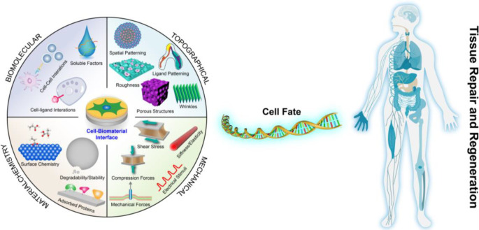
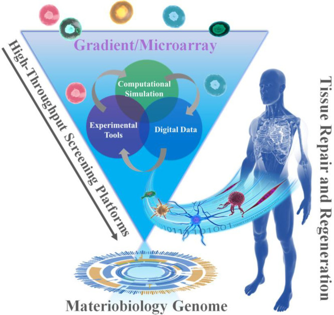
The complex interaction of cells with biomaterials (i.e., materiobiology) plays an increasingly pivotal role in the development of novel implants, biomedical devices, and tissue engineering scaffolds to treat diseases, aid in the restoration of bodily functions, construct healthy tissues, or regenerate diseased ones. However, the conventional approaches are incapable of screening the huge amount of potential material parameter combinations to identify the optimal cell responses and involve a combination of serendipity and many series of trial-and-error experiments. For advanced tissue engineering and regenerative medicine, highly efficient and complex bioanalysis platforms are expected to explore the complex interaction of cells with biomaterials using combinatorial approaches that offer desired complex microenvironments during healing, development, and homeostasis. In this review, we first introduce materiobiology and its high-throughput screening (HTS). Then we present an in-depth of the recent progress of 2D/3D HTS platforms (i.e., gradient and microarray) in the principle, preparation, screening for materiobiology, and combination with other advanced technologies. The Compendium for Biomaterial Transcriptomics and high content imaging, computational simulations, and their translation toward commercial and clinical uses are highlighted. In the final section, current challenges and future perspectives are discussed. High-throughput experimentation within the field of materiobiology enables the elucidation of the relationships between biomaterial properties and biological behavior and thereby serves as a potential tool for accelerating the development of high-performance biomaterials.

Figure 1

Variables within the cell–microenvironment interface can invoke a biological response and decide cell fate in the process of tissue repair and regeneration.

Figure 2

Schematic diagram of the interactions between cells and biointerface/matrix.

Figure 3

Schematic overview of different experimental designs for two factors x₁ and x₂, including a table of the experimental runs to be performed. (a) OAT design, (b) two-level full factorial design, (c) three-level full factorial design, (d) three-level fractional factorial design. Note that for the OAT-design it is assumed that the intermediate level (0) is the standard level. −1 refers to the low level and +1 refers to the high level of a particular factor.

Figure 4

Schematic diagram of the combinations of HT screening, materiobiology genome, as well as tissue repair and regeneration.

Figure 5

(a) Schematic illustration of a 2D surface gradient and the advantages over single sample measuring. (b) Illustration of cellular responses to a physicochemical parameter on a surface gradient.

Figure 6

Different methods for preparing stiffness gradients. (A) Schematic representations displaying the formation of PVA hydrogel with stiffness gradient by the freeze–thaw method. Reprinted with permission from ref (38). Copyright 2015 Elsevier, Ltd. (B) Schematic preparation process for PDMS stiffness gradients via a temperature gradient during curing. Reprinted with permission from ref (148). Copyright 2012 Elsevier, Ltd.

Figure 7

Schematic diagrams for preparing anisotropic gradient. (A) Arrays with varied intervals prepared by UV-assisted capillary force lithography. (a) Schematic of the preparation process for pattern arrays. (b) 3D AFM picture. (c) SEM image. Reprinted with permission from ref (160). Copyright 2009 Elsevier, Ltd. (B) (a) Procedure for the fabrication of wrinkle gradient. (b) AFM pictures along the gradient. Reprinted with permission from ref (100). Copyright 2017 American Chemical Society.

Figure 8

(A) Schematic representation displaying the preparation process of pore size gradient by a centrifugation technique. Reprinted with permission from ref (175). Copyright 2007 American Chemical Society. (B) Schematic diagrams illustrating the fabrication of PCL roughness-gradient. Reprinted with permission from ref (181). Copyright 2014 Elsevier, Ltd. (C) Schematic drawing of the dip-coating process to prepare particle gradient. Reprinted with permission from ref (186). Copyright 2007 American Chemical Society. (D) Schematic diagram for producing a density gradient of microparticles by electrospray method. Reprinted with permission from ref (189). Copyright 2010 WILEY-VCH.

Figure 9

(A) Schematic diagram for the design double orthogonal gradient composed of stiffness gradient and Fn density gradient. Reprinted with permission from ref (259). Copyright 2015 Nature Publishing Group. (B) Schematic presentation for the fabrication of an orthogonal gradient comprising pore size gradient and RGD gradient. Reprinted with permission from ref (260). Copyright 2012 Royal Society of Chemistry. (C) Formation of unidirectional single and orthogonal double surface gradients (stiffness and wettability). Reprinted with permission from ref (146). Copyright 2018 WILEY-VCH.

Figure 10

(A) (a) DNA contents of hBM-MSC grown on the stiffness gradient for different days and (b) immunofluorescence staining of hBM-MSCs after culturing for 28 days. Reprinted with permission from ref (38). Copyright 2015 Elsevier, Ltd. (B) DNA contents of hBM-MSC cultured on the stiffness gradient for different time. Reprinted with permission from ref (147). Copyright 2016 Elsevier, Ltd. (C) Fluorescent images of stained human dermal fibroblasts (HDFs) across the gradient after (a) 24 h attachment, and 6 days proliferation. (III) Cell density of HDF after (c) 1 day and (d) 6 days. Blue for cell nucleus and green for cytoskeleton. Reprinted with permission from ref (39). Copyright 2013 Elsevier, Ltd.

Figure 11

(A) (a) Fluorescent staining of the gradients. Red color is for cytoskeleton. (b) Cell macroscopic behaviors. Reprinted with permission from ref (100). Copyright 2017 American Chemical Society. (B) (a) SEM of the polycaprolactone roughness gradient. (b) F-actin staining at day 4. (c) Quantified cell perimeter along the gradient after 4 days. Reprinted with permission from ref (181). Copyright 2014 Elsevier, Ltd.

Figure 12

(A) Attachment of MSC on (a) COL1 and (b) OPN gradient after 5 h. Reprinted with permission from ref (291). Copyright 2019 WILEY-VCH. (B) Cell morphology on (a) OD–AA and (b) AA–DG gradient. Quantification for cell number after (c) 1 day and (d) 6 days. Reprinted with permission from ref (231). Copyright 2015 Elsevier, Ltd.

Figure 13

(A) Immunofluorescent staining of hBM-MSC grown on 1–24 kPa gradient after 28 days and the results for quantitation. Reprinted with permission from ref (38). Copyright 2015 Elsevier, Ltd. (B) Immunofluorescent staining of hBM-MSC grown on 20–200 kPa gradient after 2 and 4 weeks. Reprinted with permission from ref (147). Copyright 2016 Elsevier, Ltd.

Figure 14

(A) Immunostaining of Tuj1 of MSCs grown on wrinkle gradients for (a) 1 week and (c) 2 weeks. (b, d) Zoomed picture of the typical position and quantitative results of Tuj1. Reprinted with permission from ref (173). Copyright 2020 Wiley-VCH. (B) (a) Immunostaining of ALP for cells cultured on roughness gradient after 4 and 21 days. (b) Quantitative results of ALP. Reprinted with permission from ref (181). Copyright 2014 Elsevier, Ltd.

Figure 15

(A) Influence of COL1 and OPN gradient on Runx2 expression after 7 day under (a, c) osteogenic medium (OSM) and (b, d) DMEM. (e) Quantitative results of Runx2 on the COL1 and OPN gradients. Reprinted with permission from ref (291). Copyright 2019 Wiley-VCH. (B) Adipogenesis/osteogenesis on OD–AA gradient under mixed medium after 14 days. (a) Nile red staining and (b) Calcein Blue staining, respectively. (c) Quantification results along the gradient. Reprinted with permission from ref (231). Copyright 2015 Elsevier, Ltd.

Figure 16

(A) Representative migration behaviors for VSMCs cultured on the stiffness gradient and uniform stiffness gels decorated with Fn or laminin. Reprinted with permission from ref (348). Copyright 2016 National Academy of Sciences. (B) Migration trajectories of cells on an (a) densely and (c) sparsely spaced ridged arrays. The skewness of the distributions is shown in each panel (b, d). Reprinted with permission from ref (160). Copyright 2009 Elsevier, Ltd. (C) Cell migration trajectories on the swelling gradient. The arrows mean the ratios of cells moving to the direction of the lower degree of hydration. Reprinted with permission from ref (357). Copyright 2013 Elsevier, Ltd. (D) Left: Schematic representation for the structure of a complementary density gradient of PDMAPS and KHI. Right: The effect on the migration of SCs and FIBs. Reprinted with permission from ref (368). Copyright 2015 Elsevier, Ltd.

Figure 17

Illustrative workflow for high-throughput microarray studies in cellular applications (representations not to scale). First, microarray fabrication can be done through automated liquid dispensing systems (contact printing with a solid or quilled pin, or inkjet printing). Second, high-throughput is carried out for (1) material analysis technologies (e.g., time-of-flight mass spectrometry (ToF SIMS), WCA, X-ray photoelectron spectroscopy (XPS), atomic force microscopy (AFM)), and (2) biological performance. Third, biological and structural data are correlated, and used to generate structure–activity relationship models. The material library can be further mined through combinatorial microarrays of the highest performing biomaterials, and computational models can be generated from the available data sets. After extensive mining of the microarray-generated data, scale-up studies take the best-performing polymers onto bigger platforms, such as multiwell tissue culture plates, robot-assisted automated cell culture platforms using RoboFlasks, or 3D culture by generating microparticles from the hit polymers and using them in Bioreactor-based strategies. In-depth cell-based studies (e.g., proliferation assessment, transcriptional analysis, and specific cell marker immunostaining) can then be performed in parallel to investigate the long-term effect of “hit” polymers on cellular behavior. Ultimately, preclinical studies on animals, followed by clinical trials are undertaken to ensure the biomaterial’s safety and effectiveness in biomedical applications.

Figure 18

(A, B) Combinatorial strategy applied to microarray formation Reprinted with permission from ref (441). Copyright 2013 Wiley-VCH. (A) Schematic of the combinatorial design; (i) first generation array consists of 116 homopolymers, (ii) second generation array consisted of 324 copolymers formed by mixing 18 “hit” monomers pairwise, (iii) third generation array explored 13 “hit” compositions from the second generation array via incremental compositional variations, (iv) lead compositions from the third generation were selected for scale-up and additional testing. (B) Results from applying the microarray strategy from Hook et al.; (i) chemical structures of hit monomers selected from the 1st generation array; (ii) intensity scale image representing bacterial attachment averaged value (iota) for each of the materials in the 2nd generation array, the scale on the right is nonlinear to highlight the range of the array, the central square is the iota value, while the narrow columns to the left indicate standard deviation (n = 3), the major or minor monomer is indicated across the row or column, respectively; (iii) intensity scale image of the iota value for each of the materials in the third generation array, the monomers used are indicated to the left and right of the intensity scale, and refer to the monomers shown in (i), the content (%) of each of the monomers listed on the left is indicated in the top row. (C, D) Microarray fabrication. Reprinted with permission from ref (418). Copyright 2019 Elsevier, Ltd. (C) Representation of the spot-in-spot fabrication strategy, (i) ratio of monomer drops printed on each spot, (ii) schematic pattern of the printed microarray. (D) Results by Zhang et al.: (i) image of a microarray printed on a microscope slide with 28 × 87 polymer spots, (ii) corresponding fluorescent image of the spots, (iii) mosaic made with brightfield images of representative spots on the microarray, (iv) corresponding fluorescent images for the spots represented in (iii), (v) enlarged brightfield image of a feature with cells (red box in (iii)), (vi) enlarged fluorescent image of cells on a spot (red box in (iv)), scale bar = 200 μm.

Figure 19

Microarrays assessed for spot defects. Reprinted with permission from ref (443). Copyright 2013 Royal Society of Chemistry. (a) Overview of a combinatorial microarray prepared using premixed combinations of commercially available monomers and on-slide polymerization. (b) Representative images of defective copolymer spots showing noncircularity, spreading, and roughness (light microscopy), and chemical heterogeneity (ToF SIMS images of the C₃H₃^– ion); images of the corresponding nondefective homopolymers (left images); (c) AFM images of polymer spots assigned with a roughness defect. Images are 5 × 5 μm².

Figure 20

Microarray fabrication strategies for 2.5/3D microenvironment investigation. (A) Microarray production. Reprinted with permission from ref (448). Copyright 2015 Nature Publishing Group. (a) Schematic of the microarray production process, (b) human MSC viability after 7 days in culture along with a color-diagram (right) displaying the quantified cell viability per system. (B) Microarray. Reprinted with permission from ref (450). Copyright 2014 Nature Publishing Group. (c) Enzymatically mediated cross-linking scheme represents a specific peptide sequence, (d) biologically relevant factors are used to generate a combinatorial toolbox in a categorized form, (e) schematic of the experimental process: combining the components library with reporter cells (Oct4-GFP mouse ECSs) using robotic mixing and dispensing technology into 1,536 well plates, (f) representative images of automated microscopy, used to determine colony growth in every single well over a 5-day experiment, (g) 3D confocal reconstruction and (h) image segmentation using automated microscopy and computational methods; scale bar = 200 μm. (C) Microfabrication strategy. Reprinted with permission from ref (452). Copyright 2010 Elsevier, Ltd., (i) schematic representation of the fabrication process for mechanically active 3D cell culture arrays, (j) photo of the entire array connected to the solenoid valve, the green dye in the pressurized actuation channels), (k) increasing actuation cavity size across the array enables a range of mechanical conditions to be created simultaneously, (l) cylindrical hydrogel polymerized on a loading post of the active culture array.

Figure 21

Representative microarrays to investigate the effect of topographical features on cell phenotype. (A–E) TopoChip characterization. Reprinted with permission from ref (455). Copyright 2011 National Academy of Sciences. (A, B) SEM images of a section of TopoChips, displaying accurate feature replication (scale bar = 50 μm), (C) image of the TopoChip carrier, lid and chip assembly, (D, E) light microscopy images of cells seeded onto the TopoChip displaying homogeneity of cell distribution within and between TopoUnits. (F) TopoWellPlate fabrication scheme. Reprinted with permission from ref (51). Copyright 2011 Wiley-VCH. representing the following steps (a) silicon master mold containing the inverse structures of the selected topographies is used to (b) cast a layer of PDMS, followed by (c) curing of the PDMS layer and (d) peeling off from the silicon master. (e) OrmoPrime is applied to a Borofloat wafer, followed by application of OrmoStamp onto the PDMS mold, (f) which is spread by capillary forces, (g) UV curated and (h) peeled off from the mold. The hot embossing process involves (i) the inverse OrmoStamp mold is aligned (j) to the polystyrene film followed by (k) hot embossing and (l) gentle peeling off. The patterned polystyrene film is then (m) aligned to the bottomless 96-well plate and an aluminum thermal stamp, followed by (n) thermal bonding, resulting in (o) a leakage-free well plate containing defined surface substrates.

Figure 22

Strategy used by Hammad et al. From left to right: Sequential inkjet printing of biomolecules on the same coordinates as the polymer spots (in orange) in the primary screen: proteins were mixed pairwise at a 70/30% ratio and at 0.1, 0.5, and 1 fmol. Table showing results of the primary screen, displaying color coding for human PSC line (HUES7) cell number (OCT-4-positive cell quantification) per spot. A secondary microarray screen was generated from “hit” protein combinations, mixed pairwise at 30, 50, and 70% ratios and at 0.1, 0.5, 1, 2, and 4 fmol. The table shows representative results of OCT4-positive cells per spot in the second generation array. Reprinted with permission from ref (474). Copyright 2010 Royal Society of Chemistry.

Figure 23

Microarray technologies based on animal-derived biomolecules. Reprinted with permission from ref (437). Copyright 2008 Wiley-VCH. (A) Fluorescent image of a two-component protein array, composed of 25 different combinations of mini-arrays (white square marks one mini-array), red spots are Alexa-546-labeled fibrinogen and green spots are FITC-labeled BSA, the numbers at the top of representing the distance between spots and the numbers on the left are the ratio of red: green spots. (B) Collage of fluorescence images of C2C12 myoblast cell adhesion on fibronectin arrays after a 3h incubation on protein arrays with different spot spacing, (C, D) enlarged images of the red squares gown in panel B, scale bar = 20 μm. (E) Correlation between fibronectin surface coverage and cell density (black line) or cell spreading (red line). (F–I) Microarray fabrication. Reprinted with permission from ref (417). Copyright 2016 Elsevier, Ltd. (F) Schematic of the cell microarray formation, (G) Typical cell microarray platform with various protein ratios. (H) Fluorescent images of the slide acquired using automated fluorescence microscopy for nuclear localization (Hoechst 33342) and osteogenic markers (Runx2, Calcein Blue). (I) Automated analysis for the detection and measurement of nuclear count and osteogenic marker presence (yellow line in Runx2 and blue line in Calcein Blue, Ca ion). (J–L) Microarray strategy. Reprinted with permission from ref (489). Copyright 2016 Elsevier, Ltd. (J) Schematic of the experimental approach, with 4000 features (including positive and negative controls) on a single glass slide, (K) representative image of complete ECM microarray 12 h post cell-seeding with definitive endoderm cells, image represents the 4000 features in the array, nucleus and cytoplasm are labeled with fluorescent dyes (blue and green, respectively) and red spots are rhodamine-dextran spots utilized as negative controls and for alignment of image acquisition, scale bar = 1 mm. (L) Inset from panel B (white box), including cell nuclei label only and illustrating a representative set of ECM islands in quintuplicate, scale bar = 100 μm. Right graph shows a heatmap quantification of endoderm cell adhesion 12 h postseeding. Each feature represents the combination formed by 2 different ECM molecules on the x and y axes.

Figure 24

Microarray strategies for 2D/surface printing of biomolecules and synthetic polymers. (A) Schematic of the strategy. Reprinted with permission from ref (501). Copyright 2016 MDPI. First, in silico screening of candidate peptides is performed, and candidate 9-mer peptides are selected from the homologous sequences. Second, the microarray is fabricated using a peptide array synthesizer on a cellulose membrane, which is cut and deposited in a 96-well plate. Cells are seeded, cultured, and assayed for cell proliferation and osteogenic differentiation. (B) Polymer microarray. Reprinted with permission from ref (442). Copyright 2014 Royal Society of Chemistry. (a) Microarray fabrication using contact printing of monomer solution followed by UV polymerization, (b) high-throughput screening and characterization of polymer spots for (i) surface chemistry by ToF-SIMS, (ii) surface wettability using WCA, (iii) human stem cell adhesion and hit polymers with high cell attachment (inset); (c) structures of the 141 monomers used in the microarray, grouped by side-chain chemistry.

Figure 25

Microarray strategies using chemical nanopatterning. (A) Schematic representing the key steps involved in the generation of binary nanostructured hydrogels consisting of PEG substrates decorated with AuNPs and TiO₂NPs. Reprinted with permission from ref (536). Copyright 2016 American Chemical Society. (B) Microarray fabrication workflow steps: (i) parallel nanoimprint lithograph of a silicon wafer is performed using a stamp containing 16 replicates of 8 different line patterns, (ii) followed by surface treatment with plasma etching (PE) and physical vapor deposition (PVD) of Ti and Au, which leads to (iii) fabrication of multiple Si/Au nanoscale patterns within every 9 mm² areas; (iv) microwell generation around each patterned area via SU-8 photolithography, (v) chemical activation and modification of the SU-8 surfaces, and (vi) finally dispensing of a streptavidin solution on all patterned areas, followed by protein solutions (ratios of LN and VN) locally printed in duplicates for each pattern size, creating 64 combinations of nanopatterned ECM protein patterns. Representations not to scale. Reprinted with permission from ref (537). Copyright 2016 Wiley-VCH.

Figure 26

Microarray strategies to investigate cell responses to mechanical stimuli. (A–D) Evaluation of cell traction stress. (A, C) Cell traction stress (Pa) measured on the microarrays on 30 kPa (A) and 4 kPa (C) substrates on the different protein compositions, in control (DMSO) and ROCK inhibiting (Y-27623, 10 μM) media conditions. (B, D) Representative phase contrast micrographs and heat maps of traction stress for 30 kPa (B) and 4 kPa (D) substrates. Student’s t tests were performed against DMSO within each ECM combination, and data is presented as mean ± SEM with n = 3 and ≈ 20 total islands per condition (P < 0.05 (∗), P < 0.01 (∗∗), P < 0.001 (∗∗∗)). The scale bar is 50 μm. Reprinted with permission from ref (541). Copyright 2016 Elsevier, Ltd. (E–N) Microarray strategy. (E) Schematic of the overall microarray chip with zoom on a single active area and on a single pixel, (F) picture of the chip bonded on the carrier, (G) SEM image of one active area featuring the 4 different electrode sizes and the 8 reference electrodes. (H, I) SEM images of a single pixel, containing electrodes of sizes 2.5 × 3.5 μm² (H) or 11 × 11 μm² (I). (J–N) Electrical and confocal imaging of primary hippocampal neuron culture at 0 and 8 days in vitro. (J, K) Electrical impedance map and confocal image of the cells stained with Calcein AM 4.5 h after seeding. (L, M) Electrical impedance map and confocal images corresponding to the same chip surface area (2500 μm²). (N) Histogram illustrating the distribution of the relative impedance variation recorded by the electrodes for cells after 0 (black) and 8 (gray) days in vitro. Reprinted with permission from ref (551). Copyright 2019 Frontiers.

Figure 27

Magnetically actuated, cell-laden hydrogels (μMACs). Three types of masks are designed, one for each of the layers: (i) a “magnetically actuated” PEGDMA layer encapsulating magnetic Fe₃O₄ nanoparticles, (ii) a stiff, constrained layer, and (iii) a gelatin methacrylate layer encapsulating the cells. The bottom right shows a photo of the hydrogel and cells setup, scale bar = 2 mm. (B) Fluorescent confocal images (top panel) and 3D reconstructions (bottom panel) of encapsulated fibroblasts in μMACs (modulus = 6 kPa) under different strain conditions. Cellular F-actin fibers stained using phalloidin (red), and nuclei (DAPI, blue). Graphs show (left) mean cell spreading volume increase over culture time and increased strain levels, rising quickly to an asymptotic saturation level at a critical strain in the range of 40–60%, and (right) cell proliferation increases with time and strain levels, saturating at the ∼40% strain condition. Scale bars = 500 μm. Error bars, SD (n = 10 μMACs for each strain level, ∗∗P < 0.01, ∗∗∗P < 0.001). Reprinted with permission from ref (556). Copyright 2016 Nature Publishing Group.

Figure 28

Features of cell-based topographical microarrays. (A) Fluorescent images ranking surfaces by nucleus roundness of human MSCs growing on patterned PLA surfaces; the three lowest and three highest-ranked surfaces are represented. The topographies are represented and colored according to a Mann–Whitney U-test ranking. Cells show nuclear (red) and cytoskeleton (green) staining. Reprinted with permission from ref (144). Copyright 2015 Elsevier, Ltd. (B) High fidelity of PDMS patterns generated from the MARC master molds by soft lithography. SEM images of (i) unpatterned PDMS control, and (ii–viii) patterned topographies, with the description of patterned size (line width or pillar and well diameter, μm), pattern spacing (μm) and pattern height (μm), in that order. The perpendicular pattern is also indicated with the abbreviation (pr). Scale bar = 5 μm. Reprinted with permission from ref (571). Copyright 2013 Elsevier, Ltd.

Figure 29

Macrophage cell attachment is mediated by small circular pillar topography. (A) Macrophage cell attachment represented as high (blue), medium (green), or low (orange) plotted against total pattern area (μm²). Categories of macrophage attachment were determined through cluster analysis using Euclidian distance. Composite confocal images showing cell membrane (green) and nucleus (blue), representative of (B) low attachment, or (C) high attachment TopoUnits with inset (D) with orthogonal views of Z-stack images showing cellular engulfment of the cylindrical pillar feature. Scale bar = 10 μm. Reprinted with permission from ref (602). Copyright 2020 Wiley-VCH.

Figure 30

High-throughput microfluidic platforms. (A) Standard multiwell plate based-microfluidics. (a) Sliced tissue culture system for drug screening. Reprinted with permission from ref (679). Copyright 2014 Royal Society of Chemistry. (b) Multiwell plate-based 3D cell culture platform with 40 culture chambers. Reprinted with permission from ref (677). Copyright 2013 Royal Society of Chemistry. (c) A 384 hanging drop spheroid culture array plate. Reprinted with permission from ref (680). Copyright 2011 Royal Society of Chemistry. (B) Microstructure-based cell culture array. (a) Microfluidic cell culture unit for long-term cellular monitoring. Reprinted with permission from ref (636). Copyright 2005 Wiley-VCH. (b) Microfluidic device containing thousands of cell traps for cell capture and pairing. Scale bar, 20 μm. Reprinted with permission from ref (705). Copyright 2009 Nature Publishing Group. (C) Valve-assisted microfluidic platforms. (a) Integration of 96 parallel cell culture chambers on a chip. Reprinted and modified with permission from ref (638). Copyright 2007 American Chemical Society. (b) Microfluidic living cell array. Reprinted with permission from ref (728). Copyright 2007 Royal Society of Chemistry. (D) Droplet-based microfluidics. (a) Microfluidic channel array for droplet immobilization. Scale, 40 μm. Reprinted with permission from ref (734). Copyright 2009 Royal Society of Chemistry. (b) Microfluidic droplet printer for dispensing programmed combinations of cells and reagents on the substrate. Reprinted with permission from ref (737). Copyright 2017 National Academy of Sciences.

Figure 31

Concentration gradient generation in microfluidic devices. (A) Chemical concentration gradient generation on microfluidic platforms. (a) Microfluidic T-channel with two input fluids in a steady state. Reprinted with permission from ref (743). Copyright 1999 American Chemical Society. (b) Gradient culture device. Reprinted with permission from ref (746). Copyright 2015 Royal Society of Chemistry. (c) Microfluidic channel network to create the gradients of two dyes in solution. Reprinted with permission from ref (640). Copyright 2001 American Chemical Society. (d) Microfluidic high-throughput cell-based assay. Reprinted with permission from ref (636). Copyright 2005 Wiley-VCH. (e) Multilayer microfluidic device to create 3 replicates of 10 independent concentration gradients. Reprinted with permission from ref (650). Copyright 2013 Royal Society of Chemistry. (B) Oxygen concentration gradient control in microfluidic devices. (a) Microfluidic device to formulate oxygen gradients by diffusing oxygen through PDMS side walls. Reprinted with permission from ref (689). Copyright 2011 Royal Society of Chemistry. (b) Microfluidic oxygen tension generator integrated with a sandwiched gas permeable membrane. Reprinted with permission from ref (691). Copyright 2013 Royal Society of Chemistry. (C) Multiple gradients formation. (a) Microfluidic cell culture platform capable of generating chemical and oxygen gradients. Reprinted with permission from ref (749). Copyright 2014 Royal Society of Chemistry. (b) High-throughput photodynamic therapy (PDT) screening chip. Scale bar 5 mm (right). Reprinted with permission from ref (751). Copyright 2014 Royal Society of Chemistry.

Figure 32

Mechanochemical stimulation generated by microfluidic components. (A) Shear stress. (a) Cell culture array with a channel network to apply a logarithmic range of shear stress. Reprinted with permission from ref (756). Copyright 2006 Royal Society of Chemistry. (b) Microfluidic shear device with the channel embedded with ECM molecule-coated PDMS posts. Scale bars, 6 μm (right) and 20 μm (bottom left). Reprinted with permission from ref (414). Copyright 2012 Royal Society of Chemistry. (B) Compression. (a) Compression device to evaluate differentiation of hMSCs and hASCs toward osteogenesis under cyclic pneumatic force. Scale bar 100 μm. Reprinted with permission from ref (654). Copyright 2012 PLOS. (b) Microfluidic axon injury microcompression device. Scale bar 25 μm. Reprinted with permission from ref (762). Copyright 2011 Royal Society of Chemistry. (C) Stretching. (a) High-throughput cell stretcher chip combined with 9 × 12 arrays of mechanically active culture units. Reprinted and modified with permission from ref (597). Copyright 2010 Royal Society of Chemistry. (b) Microfluidic stretcher consisting of eight stretching units with nanosized posts patterned actuation cavity layer. Reprinted with permission from ref (661). Copyright 2015 Nature Publishing Group.

Figure 33

Cell culture in 3D matrices in microfluidic chips. (A) Compartmentalization. (a) Microfluidic chip for hepatocyte 3D culture and multiple drug testing. Reprinted with permission from ref (664). Copyright 2009 Royal Society of Chemistry. (b) Microfluidic device for constructing a neural circuit in 3D. Scale bar 200 μm. Reprinted with permission from ref (669). Copyright 2016 Wiley-VCH. (c) Microfluidic 3D blood capillary model using BMA-EDMA-supported hydrogel patterning. Scale bar 50 μm. Reprinted with permission from ref (670). Copyright 2018 Wiley-VCH. (B) Patterning using sacrificial elements. Fabrication process to create microfluidic channels within collagen gels (top). Photos show a device design, a fabricated device, and DAPI stained-HUVECs culture in the channel (bottom). Reprinted with permission from ref (768). Copyright 2013 Royal Society of Chemistry. (C) Molding. (a) Fabrication of PDMS/PEG-hydrogel microfluidic networks. Reprinted with permission from ref (777). Copyright 2010 Elsevier, Ltd. (b) Schematic fabrication process of hydrogel microfluidic device by a twice-cross-linking technique. Reprinted with permission from ref (772). Copyright 2018 Wiley-VCH.

Figure 34

Microfluidic organ-on-a-chip models. (A) Microfluidics-based 3D neurovascular unit platform. (a) Design of the platform to create a blood–brain barrier. (b) Fabrication steps to form the microfluidic blood–brain barrier. Reprinted with permission from ref (801). Copyright 2017 Nature Publishing Group. (B) Gut-on-a-chip microfluidic platform. (a) Device design with a porous stretchable membrane. (b) Comparison of cell shape and polarity in a static Transwell model and the recreated gut microenvironment. Scale bars, 20 μm. Reprinted with permission from ref (798). Copyright 2012 Royal Society of Chemistry. (C) 3D printed oviduct-on-a-chip platform. (a) Schematics of the device. (b) 3D cultured bovine oviduct epithelial cells (BOECs) in the device. Scale bars, 25 μm. (c) Ciliated cells at the air–liquid interface during culture. (d) On-chip monospermic oocyte penetrations. Scale bar, 50 μm. Reprinted with permission from ref (797). Copyright 2017 Royal Society of Chemistry. (D) Multiorgan-on-a-plate system. (a) Multiorgan models and microfluidic circulatory networks. (b) Assembly of the device. (c) Evaluation of three anticancer drugs in the four-organ system composed of the intestine, liver, cancer, and connective tissue models. Reprinted with permission from ref (787). Copyright 2017 Royal Society of Chemistry.

Figure 35

Cells receive stimuli from their surroundings, such as small molecules (1), the physical (i.e., surface topography, porosity, stiffness, elasticity etc.) (2) and (bio)chemical (2) and surface (bio)chemical (3) properties of a material, and produce a response via signaling pathways. The pathways can, in turn, lead to the production of transcription enhancers, such as transcription factors (4) that enable the expression of certain genes (5). This gene expression can lead to different cell phenotypes (6) such as proliferation, differentiation, or cell death.

Figure 36

Comparison of the high-throughput and high content assay readouts as reviewed by Mercola et al.

Figure 37

Single-cell, treated with either floxuridine or etoposide, show distinct image-based signatures. Adopted from Caicedo et al.

Figure 38

Workflow for assay development and image analysis for HCI, proposed by Boutros et al.

Figure 39

Main steps to extract quantitative information from images.

Figure 40

Scatterplot of cell silhouettes according to compactness and elongation values. The cells indicated using black arrowheads share similar elongation values and differ markedly in their circularity and border complexity. As quantified by Bitar et al.

Figure 41

Basic principles of data analysis: parametrization. The biomaterial is characterized by 9 features or descriptors whereas the cell response is described by 6 features or descriptors in this toy example. m/z, mass to charge ratio; #C–O, number of C or O atoms; #Δ, number of triangles present in a surface topography; #pits, number of pits present in a surface topography; gene A-B, relative gene expression versus a control; area, cell area; aspect ratio, cell aspect ratio (length/width); fluorescent intensity, the fluorescent intensity of a marker of interest.

Figure 42

Basic principles of data analysis: data exploration and statistical modeling. (A) Input and output data matrix. (B) Scatterplot of the number of cells as a function of stiffness and WCA. Every sample is one data point. (C) Hierarchical clustering of the 6 data points into a dendrogram. The dendrogram or tree can be cut at any height to determine data clusters. Cutting the tree at the highest level (dashed line) results in 2 clusters (samples 1–3–6 and 2–4–5). Cutting the tree at a lower level (broken line) results in 4 clusters (samples 1–3, 6, 2–4, and 5). (D) On the basis of stiffness, the data points can be classified into two groups: high # cells and low # cells. (E) Simple linear regression where the dependent variable Y (here: the amount of cells) is predicted using the independent variable X (here: stiffness). (F) Classification of data points into two classes (open and solid circles) with an underfitted (gray line), reasonable (black curve), and overfitted (dashed curve) decision boundaries. The overfit is influenced by one black data point (arrow) and would classify a new point (blue dot) as a solid circle, which would probably be an error. (G) Example of K-fold cross-validation with K = 5. Reprinted with permission from refs (55) and (972). Copyright 2017 Elsevier, Ltd. and 2016 Nature Publishing Group.

Figure 43

Flowchart of the modeling process, illustrated by a toy example of the influence of biomaterials on cell proliferation. a.u.: arbitrary units. Adapted from ref (988) and reprinted with permission from ref (55). Copyright 2008 Georg Thieme Verlag KG and 2017 Elsevier, Ltd.

References

1. Chen F.-M.; Liu X. Advancing Biomaterials of Human Origin for Tissue Engineering. Prog. Polym. Sci. 2016, 53, 86–168. 10.1016/j.progpolymsci.2015.02.004. - DOI - PMC - PubMed
1. Lanza R.; Langer R.; Vacanti J. P.. Principles of Tissue Engineering; Academic Press, 2011.
1. Griffith L. G.; Naughton G. Tissue Engineering--Current Challenges and Expanding Opportunities. Science (Washington, DC, U. S.) 2002, 295, 1009–1014. 10.1126/science.1069210. - DOI - PubMed
1. Vacanti J. P.; Langer R. Tissue Engineering: The Design and Fabrication of Living Replacement Devices for Surgical Reconstruction and Transplantation. Lancet 1999, 354, S32–S34. 10.1016/S0140-6736(99)90247-7. - DOI - PubMed
1. Huang G.; Li F.; Zhao X.; Ma Y.; Li Y.; Lin M.; Jin G.; Lu T. J.; Genin G. M.; Xu F. Functional and Biomimetic Materials for Engineering of the Three-Dimensional Cell Microenvironment. Chem. Rev. 2017, 117, 12764–12850. 10.1021/acs.chemrev.7b00094. - DOI - PMC - PubMed
Publication types
Substances
LinkOut - more resources