Synaptic plasticity as Bayesian inference

Abstract

Learning, especially rapid learning, is critical for survival. However, learning is hard; a large number of synaptic weights must be set based on noisy, often ambiguous, sensory information. In such a high-noise regime, keeping track of probability distributions over weights is the optimal strategy. Here we hypothesize that synapses take that strategy; in essence, when they estimate weights, they include error bars. They then use that uncertainty to adjust their learning rates, with more uncertain weights having higher learning rates. We also make a second, independent, hypothesis: synapses communicate their uncertainty by linking it to variability in postsynaptic potential size, with more uncertainty leading to more variability. These two hypotheses cast synaptic plasticity as a problem of Bayesian inference, and thus provide a normative view of learning. They generalize known learning rules, offer an explanation for the large variability in the size of postsynaptic potentials and make falsifiable experimental predictions.

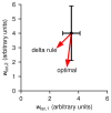
Figure 1

The delta rule is suboptimal. The error bars denote uncertainty (measured by the standard deviation around the mean) in two synapses' estimates of their target weights, w_tar,1 and w_tar,2. The first is reasonably certain; the second less so. The red arrows denote possible changes in response to a negative feedback signal. The arrow labeled “delta rule” represents an equal decrease in the first and second target weights. In contrast, the arrow labeled “optimal” takes uncertainty into account, so there is a larger change in the second, more uncertain, target weight.

Figure 2

Bayesian learning rules track the target weight and estimate uncertainty. The black line is the target weight, the red line is the mean of the inferred distribution, and the red area represents 95% confidence intervals of the inferred distribution. Panels a-c correspond to the highest presynaptic firing rate used in the simulations; panels d-f to the lowest. Consistent with our analysis (see in particular Eq. 9), higher presynaptic firing rate resulted in lower uncertainty. a and d. Linear feedback, f_lin = δ + ξ_δ. b and e. Cerebellar learning, f_cb = Θ (δ + ξ_δ − θ). c and f. Reinforcement learning, f_rl = − |δ +ξ_δ|. See Supplementary Math Note, Sec. S3, for simulation details. Note while the red lilnes are all plotted at the same thickness, the greater variability in the lower plots may make those lines appear thicker.

Figure 3

Bayesian learning rules exhibit lower error than classical ones. Red: mean squared error between the target and actual membrane potential for the Bayesian learning rules; black: mean squared error for the classical rules. a. Linear feedback, f_lin = δ + ξ_δ. b. Cerebellar learning, f_cb = Θ (δ + ξ_δ − θ). c. Reinforcement learning, f_rl = −|δ + ξ_δ|. See Supplementary Math Note, Sec. S3, for simulation details.

Figure 4

Recurrent neural network. a. Schematic of the circuit. I(t) is the input (used to initialize activity) and w corresponds to the learned output weights. The feedback weights (black arrows from V to the recurrent network) are fixed, as are the recurrent weights. During learning, the output of the network, V(t), is compared to the target output, V_tar(t), and the error is used to update the output weights, w. At test time, the target output is not fed back to the circuit. b. Learning curves, measured using mean squared error, for Bayesian and classical learning rules (red and blue, respectively, at a range of learning rates for the classical rule). Although the initial improvement in performance for the Bayesian and classical learning rules was about the same, after 100 time steps Bayesian learning became much more efficient. The arrows correspond to the number of time steps used for the comparison in panel c. c. Mean squared error versus the learning rate of the classical rule. Solid lines: classical learning rules; dashed lines: Bayesian learning rules. The mean squared error for the Bayesian learning rule was about an order of magnitude smaller than for the classical one. In panels c and d we plot the median, taken over n = 400 network/target pairs; error bars are 95% confidence intervals, computed using the percentile bootstrap.

Figure 5

Normalized variability (the ratio of the PSP variance to the mean) versus presynaptic firing rate as a diagnostic of our theory; data supplied to us by the authors of [15] (see Supplementary Math Note, Sec. S4.4). The red line, which has a slope of –1/2, is our prediction (the intercept, for which we do not have a prediction, was chosen to give the best fit to the data). The blue line is fit by linear regression(n =136 points), and the gray region represents 2 standard errors. The slope of the blue line, −0.62, is statistically significantly different from 0 (p < 0.003, t-test) and not significantly different from −1/2 (p = 0.57, t-test; assumes normality which was not formally tested). The firing rate was measured by taking the average signal from a spike deconvolution algorithm [45]. Units are arbitrary because the scale factor relating the average signal from the deconvolution algorithm and the firing rate is not exactly one [46]. Data from layer 2/3 of mouse visual cortex [15].

References

1. Poggio T. Cold Spring Harbor Symposia on Quantitative Biology. Vol. 55. Cold Spring Harbor Laboratory Press; 1990. A theory of how the brain might work. - PubMed
1. Knill DC, Richards W. Perception as Bayesian Inference. Cambridge University Press; 1996.
1. Pouget A, et al. Probabilistic brains: knowns and unknowns. Nature Neuroscience. 2013;16(9):1170–1178. doi: 10.1038/nn.3495. - DOI - PMC - PubMed
1. Aitchison L. Bayesian filtering unifies adaptive and non-adaptive neural network optimization methods. NeurIPS. 2020
1. Tripathy SJ, et al. Brain-wide analysis of electrophysiological diversity yields novel categorization of mammalian neuron types. Journal of Neurophysiology. 2015;113(10):3474–3489. doi: 10.1152/jn.00237.2015. - DOI - PMC - PubMed
Publication types
LinkOut - more resources