Universal theory of brain waves: from linear loops to nonlinear synchronized spiking and collective brain rhythms

Abstract

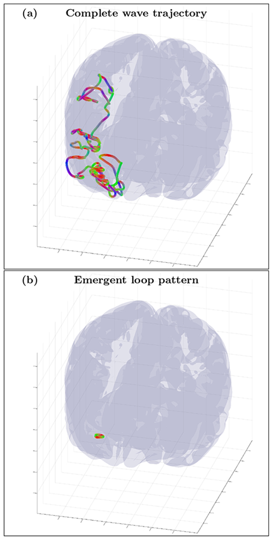
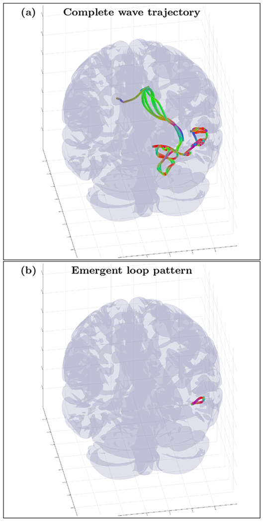
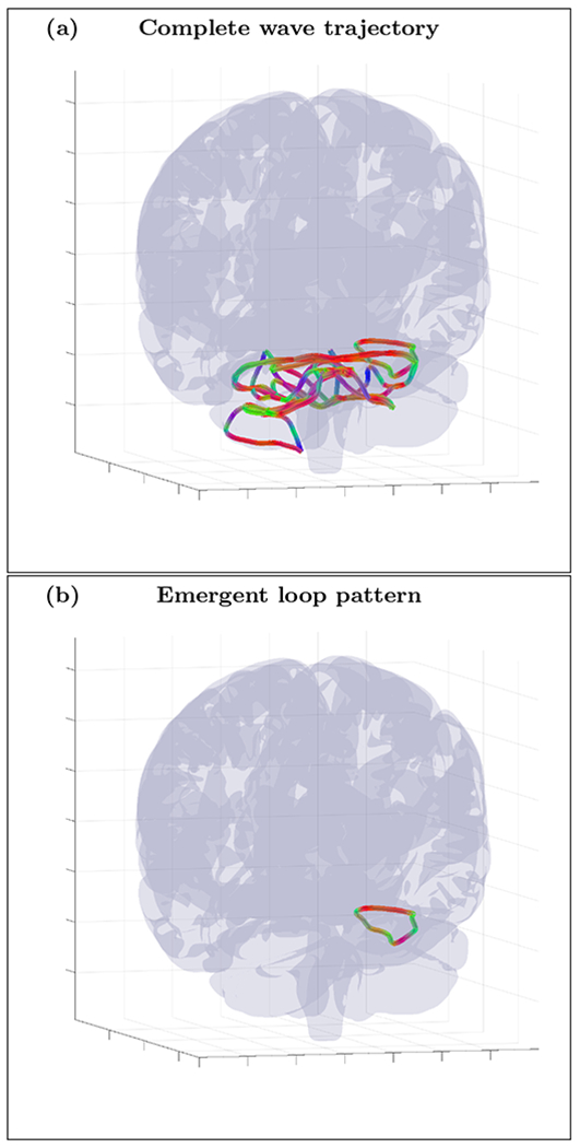
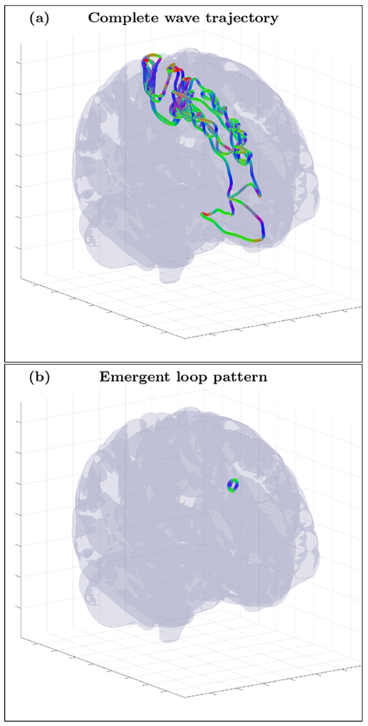
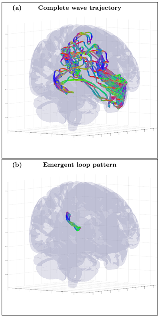
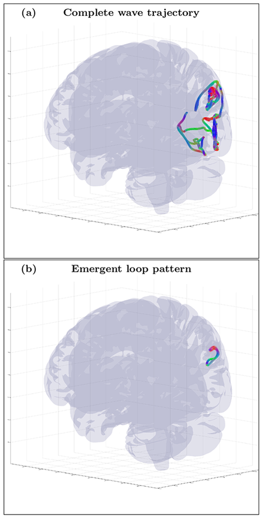
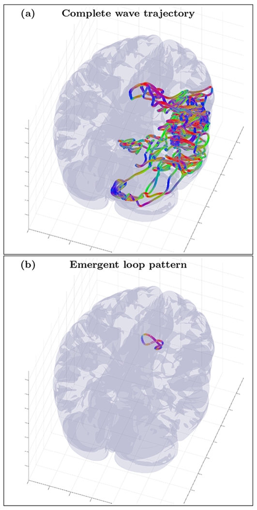
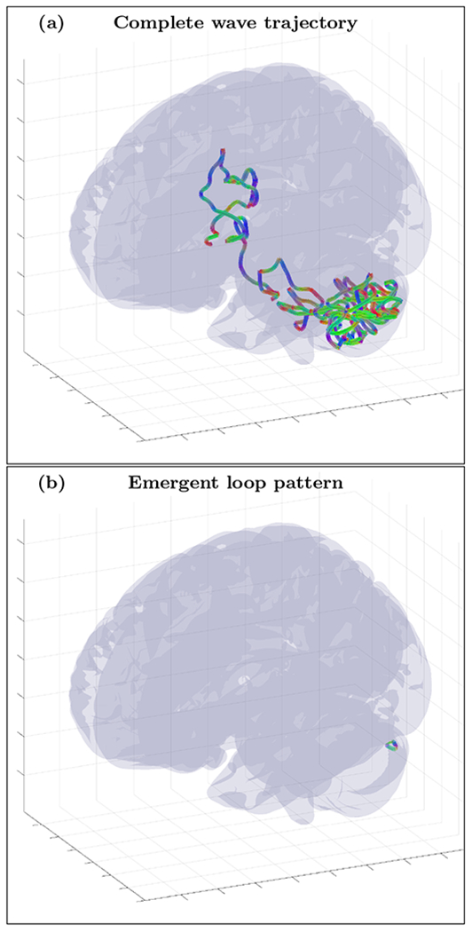
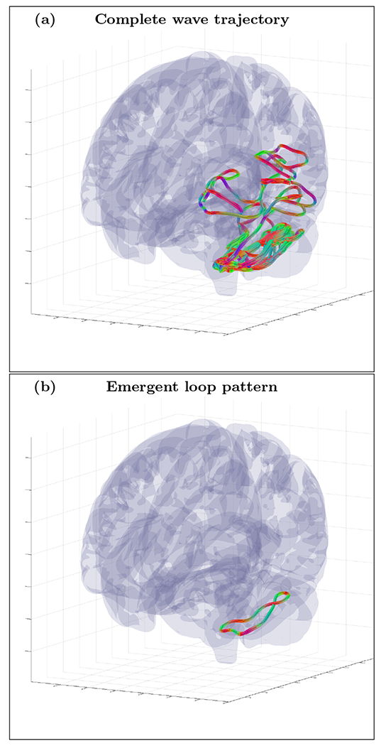
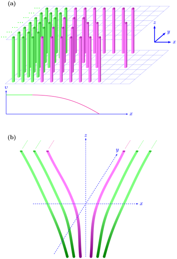
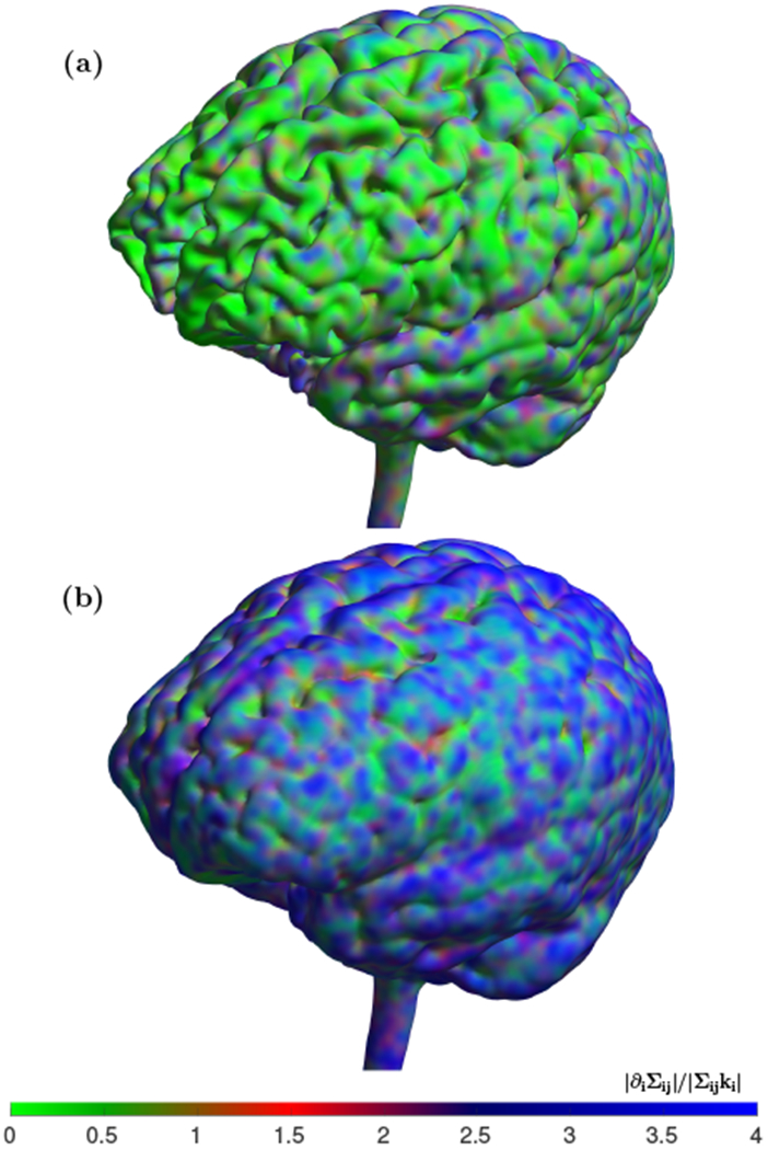
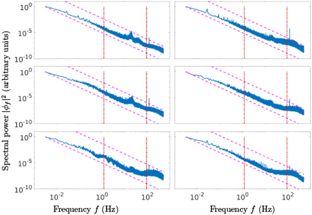
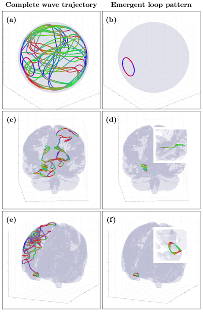
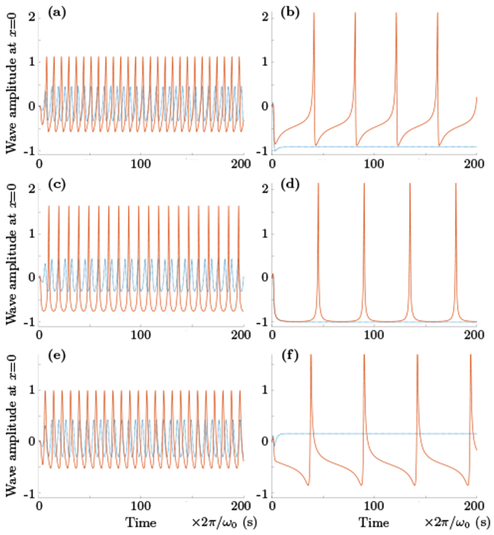
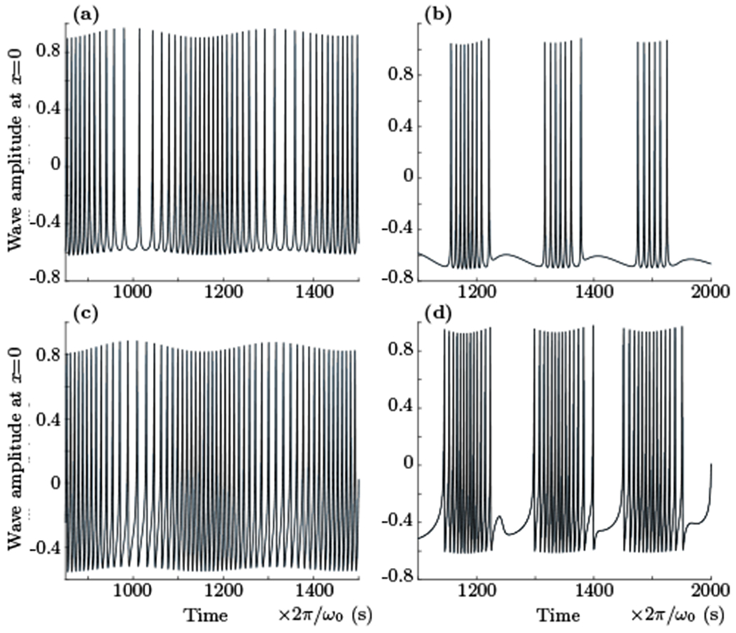
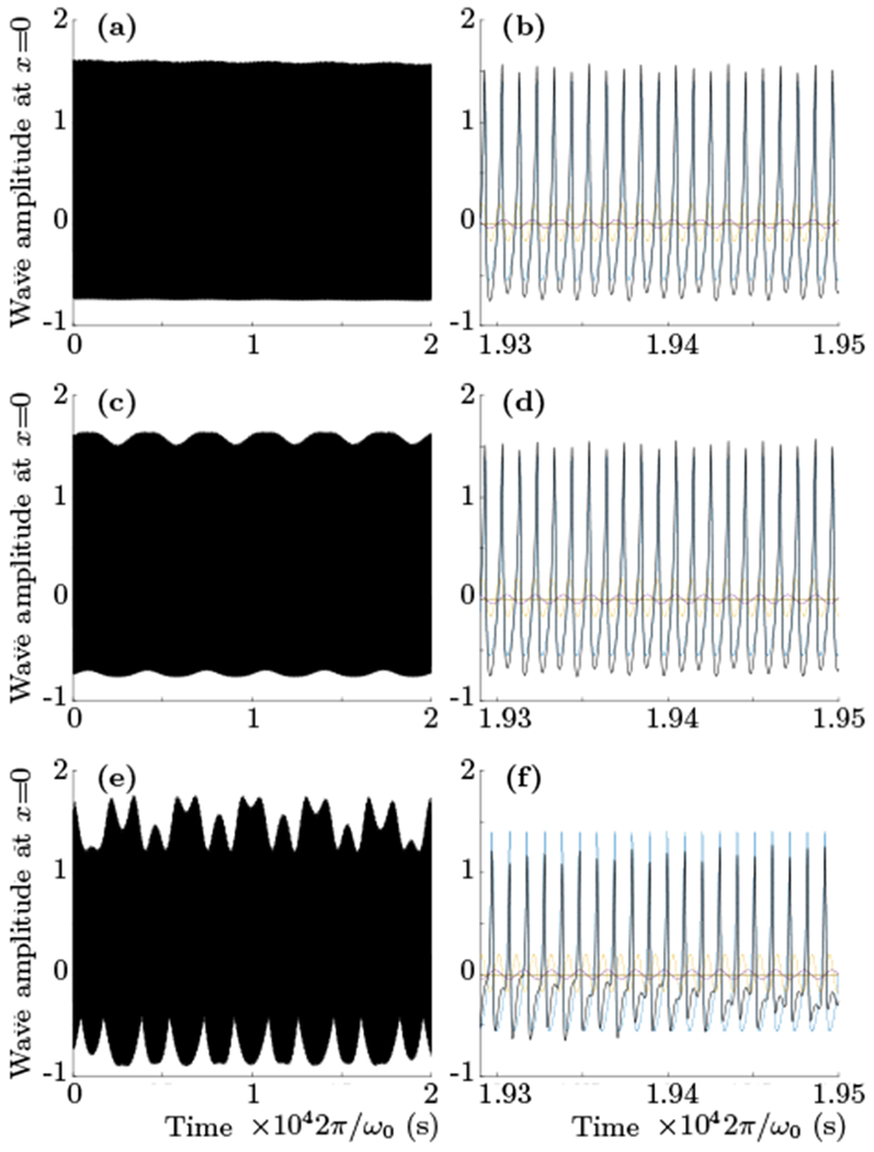
An inhomogeneous anisotropic physical model of the brain cortex is presented that predicts the emergence of non-evanescent (weakly damped) wave-like modes propagating in the thin cortex layers transverse to both the mean neural fiber direction and to the cortex spatial gradient. Although the amplitude of these modes stays below the typically observed axon spiking potential, the lifetime of these modes may significantly exceed the spiking potential inverse decay constant. Full brain numerical simulations based on parameters extracted from diffusion and structural MRI confirm the existence and extended duration of these wave modes. Contrary to the standard paradigm that the neural fibers determine the pathways for signal propagation in the brain, the signal propagation due to the cortex wave modes in highly folded areas will exhibit no apparent correlation with the fiber directions. The results are consistent with numerous recent experimental animal and human brain studies demonstrating the existence of electrostatic field activity in the form of traveling waves (including studies where neuronal connections were severed) and with wave loop induced peaks observed in EEG spectra. In addition, we demonstrate that the resonant and non-resonant terms of the nonlinear coupling between multiple modes produce both synchronous spiking-like high frequency wave activity as well as low frequency wave rhythms as a result of their unique dispersion properties. Numerical simulation of forced multiple mode dynamics shows that as forcing increases there is a transition from damped to oscillatory regime that subsequently decays away as over-excitation is reached. The resonant nonlinear coupling results in the emergence of low frequency rhythms with frequencies that are several orders of magnitude below the linear frequencies of modes taking part in the coupling. The localization and persistence of these cortical wave modes, and this new mechanism for understanding the nature of spiking behavior, have significant implications in particular for neuroimaging methods that detect electromagnetic physiological activity, such as EEG and MEG, and in general for the understanding of brain activity, including mechanisms of memory.

FIG. 9.

Plot of ρ(r) for different n

FIG. 10.

An example of complete wave trajectory (a) and emergent loop pattern (b) for the spherical shell cortex model with crossing fibers anisotropy tensor σ⁽³⁾ and narrow inhomogeneity layer (n=0, r₀=0.5 and r₁=0.9). The trajectory was initialized with wave vector $k=(-0.1/\sqrt{2},0.1/\sqrt{2},-0.1)$ inside the inhomogeneous layer with voxel coordinates r=(142,142,142). High resolution movie links: S1-H1/S1-H1, S1-H2/S1-H2. Low resolution movie links: S1-L1/S1-L1, S1-L2/S1-L2.

FIG. 11.

An example of complete wave trajectory (a) and emergent loop pattern (b) for the spherical shell cortex model with crossing fibers anisotropy tensor σ⁽³⁾ and slightly wider inhomogeneity layer (n=2, r₀=0.5 and r₁=0.9). The trajectory was initialized with wave vector $k=(-0.1/\sqrt{2},0.1/\sqrt{2},-0.1)$ inside the inhomogeneous layer with voxel coordinates r=(80,33,100). High resolution movie links: S2-H1/S2-H1, S2-H2/S2-H2. Low resolution movie links: S2-L1/S2-L1, S2-L2/S2-L2.

FIG. 12.

An example of complete wave trajectory (a) and emergent loop pattern (b) for the spherical shell cortex model with 45° orientation single fiber anisotropy tensor σ⁽²⁾ and wide inhomogeneity layer (n=25, r₀=0.5 and r₁=0.9). The trajectory was initialized with wave vector $k=(-0.1/\sqrt{2},0.1/\sqrt{2},-0.1)$ inside the inhomogeneous layer with voxel coordinates r=(145,145,145). High resolution movie links: S3-H1/S3-H1, S3-H2/S3-H2. Low resolution movie links: S3-L1/S3-L1, S3-L2/S3-L2.

FIG. 13.

An example of complete wave trajectory (a) and emergent loop pattern (b) for the spherical shell cortex model with 45° orientation single fiber anisotropy tensor σ⁽²⁾ and intermediately wide inhomogeneity layer (n=14, r₀=0.5 and r₁=0.9). The trajectory was initialized with wave vector $k=(-0.1/\sqrt{2},0.1/\sqrt{2},-0.1)$ inside the inhomogeneous layer with voxel coordinates r=(141,141,141). High resolution movie links: S4-H1/S4-H1, S4-H2/S4-H2. Low resolution movie links: S4-L1/S4-L1, S4-L2/S4-L2.

FIG. 14.

An example of randomly initialized complete wave trajectory (a) and emergent loop pattern (b) for the cortical fold model with inhomogeneity extracted from HRA volume registered to MNI152 space and with diffusion MRI derived position dependent anisotropy tensor ${\mathit{R}}^T{\mathit{\sigma }}^{(1)}\mathit{R}(\epsilon =({\lambda }_d^{(2)}+{\lambda }_d^{(3)})/2/{\lambda }_d^{(1)})$. The trajectory was initialized with wave vector k=(−0.75, 0.23, −0.62) inside the inhomogeneous layer with voxel coordinates r=(55,130,130). High resolution movie links: S5-H1/S5-H1, S5-H2/S5-H2, S5-H3/S5-H3. Low resolution movie links: S5-L1/S5-L1, S5-L2/S5-L2, S5-L3/S5-L3.

FIG. 15.

An example of randomly initialized complete wave trajectory (a) and emergent loop pattern (b) for the cortical fold model with inhomogeneity extracted from HRA volume registered to MNI152 space and with diffusion MRI derived position dependent anisotropy tensor ${\mathit{R}}^T{\mathit{\sigma }}^{(1)}\mathit{R}(\epsilon =({\lambda }_d^{(2)}/{\lambda }_d^{(1)})$. The trajectory was initialized with wave vector k=(−0.9,0.24,0.36) inside the inhomogeneous layer with voxel coordinates r=(66,94,126). High resolution movie links: S6-H1/S6-H1, S6-H2/S6-H2, S6-H3/S6-H3. Low resolution movie links: S6-L1/S6-L1, S6-L2/S6-L2, S6-L3/S6-L3.

FIG. 16.

An example of randomly initialized complete wave trajectory (a) and emergent loop pattern (b) for the cortical fold model with inhomogeneity extracted from HRA volume registered to MNI152 space and with diffusion MRI derived position dependent anisotropy tensor ${\mathit{R}}^T{\mathit{\sigma }}^{(1)}\mathit{R}({\sigma }_{22}^{(1)}={\lambda }_d^{(2)}/{\lambda }_d^{(1)}$ and ${\sigma }_{11}^{(1)}={\lambda }_d^{(3)}/{\lambda }_d^{(1)}$). The trajectory was initialized with wave vector k=(−0.77,−0.63,0.11) inside the inhomogeneous layer with voxel coordinates r=(49,153,97). High resolution movie links: S7-H1/S7-H1, S7-H2/S7-H2, S7-H3/S7-H3. Low resolution movie links: S7-L1/S7-L1, S7-L2/S7-L2, S7-L3/S7-L3.

FIG. 17.

An example of randomly initialized complete wave trajectory (a) and emergent loop pattern (b) for the cortical fold model with inhomogeneity extracted from HRA volume registered to MNI152 space and with fixed anisotropy tensor σ⁽¹⁾ (ε = 0.1). The trajectory was initialized with wave vector k=(0.56,0.58,−0.59) inside the inhomogeneous layer with voxel coordinates r=(72,156,120). High resolution movie links: S8-H1/S8-H1, S8-H2/S8-H2, S8-H3/S8-H3. Low resolution movie links: S8-L1/S8-L1, S8-L2/S8-L2, S8-L3/S8-L3.

FIG. 18.

An example of randomly initialized complete wave trajectory (a) and emergent loop pattern (b) for the cortical fold model with inhomogeneity extracted from HRA volume registered to MNI152 space and with diffusion MRI derived position independent anisotropy tensor R^T σ⁽¹⁾ R (ε = 0.1). The trajectory was initialized with wave vector k=(−0.13,−0.97,−0.21) inside the inhomogeneous layer with voxel coordinates r=(111,103,110). High resolution movie links: S9-H1/S9-H1, S9-H2/S9-H2, S9-H3/S9-H3. Low resolution movie links: S9-L1/S9-L1, S9-L2/S9-L2, S9-L3/S9-L3.

FIG. 19.

An example of randomly initialized complete wave trajectory (a) and emergent loop pattern (b) for the cortical fold model with inhomogeneity extracted from HRA volume registered to MNI152 space and with fixed anisotropy tensor σ⁽¹⁾ (ε = 0.01). The trajectory was initialized with wave vector k=(0.42,−0.41,0.81) inside the inhomogeneous layer with voxel coordinates r=(114,85,22). High resolution movie links: S10-H1/S10-H1, S10-H2/S10-H2, S10-H3/S10-H3. Low resolution movie links: S10-L1/S10-L1, S10-L2/S10-L2, S10-L3/S10-L3.

FIG. 20.

An example of randomly initialized complete wave trajectory (a) and emergent loop pattern (b) for the cortical fold model with inhomogeneity extracted from HRA volume registered to MNI152 space and with fixed anisotropy tensor σ⁽²⁾ (ε = 0.1). The trajectory was initialized with wave vector k=(−0.90,0.24,0.36) inside the inhomogeneous layer with voxel coordinates r=(66,86,126). High resolution movie links: S11-H1/S11-H1, S11-H2/S11-H2, S11-H3/S11-H3. Low resolution movie links: S11-L1/S11-L1, S11-L2/S11-L2, S11-L3/S11-L3.

FIG. 21.

An example of randomly initialized complete wave trajectory (a) and emergent loop pattern (b) for the cortical fold model with inhomogeneity extracted from HRA volume registered to MNI152 space and with diffusion MRI derived position independent anisotropy tensor R^T σ⁽¹⁾ R (ε = 0.01). The trajectory was initialized with wave vector k=(−0.90,0.24,0.36) inside the inhomogeneous layer with voxel coordinates r=(66,87,126). High resolution movie links: S12-H1/S12-H1, S12-H2/S12-H2, S12-H3/S12-H3. Low resolution movie links: S12-L1/S12-L1, S12-L2/S12-L2, S12-L3/S12-L3.

FIG. 22.

An example of randomly initialized complete wave trajectory (a) and emergent loop pattern (b) for the cortical fold model with inhomogeneity extracted from HRA volume registered to MNI152 space and with tractography derived anisotropy tensor $1/N{\Sigma }_k{\mathit{R}}_k^T{\mathit{\sigma }}^{(1)}{\mathit{R}}_k(\epsilon =0.001)$. The trajectory was initialized with wave vector k=(0.4,−0.83,0.4) inside the inhomogeneous layer with voxel coordinates r=(75,61,90). High resolution movie links: S13-H1/S13-H1, S13-H2/S13-H2, S13-H3/S13-H3. Low resolution movie links: S13-L1/S13-L1, S13-L2/S13-L2, S13-L3/S13-L3.

FIG. 23.

An example of randomly initialized complete wave trajectory (a) and emergent loop pattern (b) for the cortical fold model with inhomogeneity extracted from HRA volume registered to MNI152 space and with tractography derived anisotropy tensor $1/N{\Sigma }_k{\mathit{R}}_k^T{\mathit{\sigma }}^{(1)}{\mathit{R}}_k(\epsilon =0.01)$. The trajectory was initialized with wave vector k=(0.66,0.5,0.56) inside the inhomogeneous layer with voxel coordinates r=(33,77,56). High resolution movie links: S14-H1/S14-H1, S14-H2/S14-H2, S14-H3/S14-H3. Low resolution movie links: S14-L1/S14-L1, S14-L2/S14-L2, S14-L3/S14-L3.

FIG. 24.

An example of randomly initialized complete wave trajectory (a) and emergent loop pattern (b) for the cortical fold model with inhomogeneity extracted from HRA volume registered to MNI152 space and with tractography derived anisotropy tensor $1/N{\Sigma }_k{\mathit{R}}_k^T{\mathit{\sigma }}^{(1)}{\mathit{R}}_k(\epsilon =0.1)$. The trajectory was initialized with wave vector k=(0.36,0.67,−0.65) inside the inhomogeneous layer with voxel coordinates r=(77,123,64). High resolution movie links: S15-H1/S15-H1, S15-H2/S15-H2, S15-H3/S15-H3. Low resolution movie links: S15-L1/S15-L1, S15-L2/S15-L2, S15-L3/S15-L3.

FIG. 25.

An example of randomly initialized complete wave trajectory (a) and emergent loop pattern (b) for the cortical fold model with inhomogeneity extracted from HRA volume registered to MNI152 space and with tractography derived anisotropy tensor $1/N{\Sigma }_k{\mathit{R}}_k^T{\mathit{\sigma }}^{(1)}{\mathit{R}}_k(\epsilon =0)$. The trajectory was initialized with wave vector k=(−0.06,0.38,0.92) inside the inhomogeneous layer with voxel coordinates r=(132,113,96). High resolution movie links: S16-H1/S16-H1, S16-H2/S16-H2, S16-H3/S16-H3. Low resolution movie links: S16-L1/S16-L1, S16-L2/S16-L2, S16-L3/S16-L3.

FIG. 1.

(a) Schematic picture of half-plane packing of fibers. The uniform area of fibers oriented along z direction (shown in green) is bounded by a thin transitional area (magenta) where the conductivity gradient may be important (a sketch of one possible conductivity profile is shown at the bottom of panel). (b) Schematic picture that can be used as a crude two dimensional approximation of a fold. The direction of fiber conductivity has only x and z components and all quantities are assumed to be uniform in y direction.

FIG. 2.

Isovolume maps for comparison of dissipation vs wave-like effects at different cortex layers. (a) The isosurface from the cortex area that may be representative of white–gray matter interface. (b) The isosurface that is located in the outer cortex area of gray matter. The color scheme uses shades of green to mark regions where dissipative term dominates, i.e. |Σ_ijk_i| ≥ |∂_iΣ_ij|, shades of red where |Σ_ijk_i| < |∂_iΣ_ij| ≤ 2|Σ_ij k_i|, and shades of blue where the wave-like term is more than two times dominant, i.e. 2|Σ_ijk_i| < |∂_iΣ_ij|. The inner cortex shown in (a) clearly display prevalence of dissipation, whereas the outer cortex shown in (b) allows for wave–like cortex activity in a majority of the locations.

FIG. 3.

Spectral power of EEG signal collected with 64 sensor array and averaged over all sensors for six independent subjects is shown in six panels. The dashed lines outline the predicted f⁻² in the lower (f ≲ 1.2Hz) and higher (f ≳ 92Hz) parts of the spectra. The dashed-dotted vertical lines denote the frequency range where the cortical wave loops may be generated. Both the slope and the range agree very well with typically observed values.

FIG. 4.

Complete wave packet trajectory snapshots (left column) and emergent stable wave loop patterns (right column) for the thin spherical shell cortex model (a and b) and for the realistic cortex fold geometry (c,d,e and f). All wave packets were initialized with random parameters assuming the presence of spiky activation sources (not shown). Movie files for these and additional loop examples can be found in [21].

FIG. 5.

The results of numerical integration of the system (31) and (32), that is time evolution of potential ϕ(x, t) at x = 0 or A(t) cos(B(t) + ω_k0t). For all plots the values of ω_k0, k₀, α and β were set to be equal to 1, δ_A = 0, and γ and δ_B were varied. The top,middle and bottom rows show plots for phase delay δ_B equals to 3π/4, π/2 and π/4 respectively. The left columnn displays transformation from weakly nonlinear oscillations shown by blue dotted lines for γ = 0.75 to more strongly nonlinear regime (solid line, γ = 1.5 (top and bottom) and 2.25 (middle)). The right column shows the strongest nonlinear spiking–like time evolution of potential ϕ (solid line, γ = 2.55 (top and bottom) and 2.96 (middle)) and its transformation to non-oscillatory (blue dotted line) regime for γ = 3 (time and amplitude units are arbitrary).

FIG. 6.

The results of numerical integration of the system (31) and (32) when exponential term was replaced by I^nR integrals (28) with the region of integration set to 50k₀ < k < 1000k₀. For all plots the values of ω_k0, k₀, α and β were set to be equal to 1, δ_A = 0, and γ and δ_B were varied. The top and bottom rows show plots for phase delay δ_B equals to 3π/4 and π/2 respectively. The left column displays modulation of spiking rate for γ = 4.5. The right column shows the nonlinear bursting of spikes for γ = 5.1 (time and amplitude units are arbitrary).

FIG. 7.

The results of numerical integration of the system (35) for different values of weak resonant coupling λ = 0.001, 0.01,0.05 (top, middle and bottom rows respectively). For all plots the values of ω_k0, k₀, α and β were set to be equal to 1, and δ_A = δ_B = δ = 3π/4. The value of γ is 1.535, that is sufficiently far from the criticality, but nevertheless large enough to modify an effective period for k₀ mode to be close to that of k₁. The total potential ϕ is plotted with the black and different colors show the oscillations of the individual modes. All plots clearly show emergence of low-frequency component as a result of increase of weak resonant coupling (time and amplitude units are arbitrary).

FIG. 8.

The results of numerical integration of the system (35). For all plots the values of ω_k0, k₀, α and β were set to be equal to 1 and the resonant coupling λ was 0.05. Different values of δ were again used in real and imaginary parts (as in (31) and (32)) with δ_A = 3π/4, 0, 0, δ_B = 3π/4, 3π/4, π/2 and close to the critical values of γ = 1.731, 2.575, 2, 9969 for the left, middle and right columns respectively. The total potential ϕ is plotted with the black and different colors show the oscillations of the individual modes. All plots show that when γ is sufficiently close to criticality a week coupling produces jumps from subcritical to supercritical regimes with amazingly regular low–frequency quasiperiodicity (time and amplitude units are arbitrary).

References

1. Monai H, Inoue M, Miyakawa H, and Aonishi T, Low-frequency dielectric dispersion of brain tissue due to electrically long neurites, Phys Rev E Stat Nonlin Soft Matter Phys 86, 061911 (2012); - PubMed
2. Ingber L and Nunez PL, Neocortical dynamics at multiple scales: EEG standing waves, statistical mechanics, and physical analogs, Math Biosci 229, 160 (2011). - PubMed
1. Li XP, Xia Q, Qu D, Wu TC, Yang DG, Hao WD, Jiang X, and Li XM, The Dynamic Dielectric at a Brain Functional Site and an EM Wave Approach to Functional Brain Imaging, Scientific Reports 4, 6893 (2014); - PMC - PubMed
2. Zalesky A, Fornito A, Cocchi L, Gollo LL, and Breakspear M, Time-resolved resting-state brain networks, Proc. Natl. Acad. Sci. U.S.A 111, 10341 (2014). - PMC - PubMed
1. Van Essen DC, Smith SM, Barch DM, Behrens TEJ, Yacoub E, Ugurbil K, and for the WU-Minn HCP Consortium, The WU-Minn Human Connectome Project: An overview., NeuroImage 80, 62 (2013). - PMC - PubMed
1. Tuch DS, Wedeen VJ, Dale AM, George JS, and Belliveau JW, Conductivity Mapping of Biological Tissue Using Diffusion MRI, Annals of the New York Academy of Sciences 888, 314 (1999); - PubMed
2. Haueisen J, Tuch DS, Ramon C, Schimpf PH, Wedeen VJ, George JS, and Belliveau JW, The influence of brain tissue anisotropy on human EEG and MEG, NeuroImage 15, 159 (2002); - PubMed
3. Hallez H, Vanrumste B, Hese PV, D’Asseler Y, Lemahieu I, and de Walle RV, A finite difference method with reciprocity used to incorporate anisotropy in electroencephalogram dipole source localization, Physics in Medicine & Biology 50, 3787 (2005). - PubMed
1. Nunez PL and Srinivasan R, Neocortical dynamics due to axon propagation delays in cortico-cortical fibers: EEG traveling and standing waves with implications for top-down influences on local networks and white matter disease, Brain Res. 1542, 138 (2014). - PMC - PubMed
LinkOut - more resources