An Introductory Review of Deep Learning for Prediction Models With Big Data

Abstract

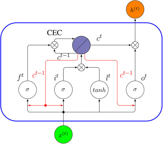
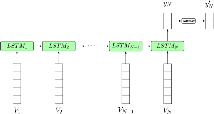
Deep learning models stand for a new learning paradigm in artificial intelligence (AI) and machine learning. Recent breakthrough results in image analysis and speech recognition have generated a massive interest in this field because also applications in many other domains providing big data seem possible. On a downside, the mathematical and computational methodology underlying deep learning models is very challenging, especially for interdisciplinary scientists. For this reason, we present in this paper an introductory review of deep learning approaches including Deep Feedforward Neural Networks (D-FFNN), Convolutional Neural Networks (CNNs), Deep Belief Networks (DBNs), Autoencoders (AEs), and Long Short-Term Memory (LSTM) networks. These models form the major core architectures of deep learning models currently used and should belong in any data scientist's toolbox. Importantly, those core architectural building blocks can be composed flexibly-in an almost Lego-like manner-to build new application-specific network architectures. Hence, a basic understanding of these network architectures is important to be prepared for future developments in AI.

Keywords: artificial intelligence; data science; deep learning; machine learning; neural networks; prediction models.

Figure 1

Number of publications in dependence on the publication year for DL, deep learning; CNN, convolutional neural network; DBN, deep belief network; LSTM, long short-term memory; AEN, autoencoder; and MLP, multilayer perceptron. The legend shows the search terms used to query the Web of Science publication database. The two dashed lines are scaled by a factor of 5 (deep learning) and 3 (convolutional neural network).

Figure 2

(A) Representation of a mathematical artificial neuron model. The input to the neuron is summed up and filtered by activation function ϕ (for examples see Table 1). (B) Simplified Representation of an artificial neuron model. Only the key elements are depicted, i.e., the input, the output, and the weights.

Figure 3

Two examples for Feedforward Neural Networks. (A) A shallow FFNN. (B) A Deep Feedforward Neural Network (D-FFNN) with 3 hidden layers.

Figure 4

(A) An example for a Convolutional Neural Network. The red edges highlight the fact that hidden layers are connected in a “local” way, i.e., only very few neurons connect the succeeding layers. (B) An example for shared weights and local connectivity in CNN. The red edges highlight the fact that hidden layers are connected in a “local” way, i.e., only very few neurons connect the succeeding layers. The labels w₁,w₂,w₃ indicate the assigned weight for each connection, three hidden nodes share the same set of weights w₁,w₂,w₃ when connecting to three local patches.

Figure 5

An example for calculating the values in the activation map. Here, the stride is 1 and the zero-padding is 0. The kernel slides by 1 pixel at a time from left to right starting from the left top position, after reaching the boarder the kernel will start from the second row and repeat the process until the whole input is covered. The red area indicates the local patch to be convoluted with the kernel, and the result is stored in the green field in the activation map.

Figure 6

Inception block structure. Here multiple blocks are stacked on top of each other, forming the input layer for the next block.

Figure 7

The structure of a residual block. Inside a block there can be as many weight layers as desired.

Figure 8

Examples for Boltzmann Machines. (A) The neurons are arranged on a circle. (B) The neurons are separated according to their type. Both Boltzmann Machines are identical and differ only in their visualization. (C) Transition from a Boltzmann Machine (left) to a Restricted Boltzmann Machine (right).

Figure 9

(A) Contrastive Divergence k-step algorithm using Gibbs sampling. (B) Backpropagation algorithm. (C) iRprop⁺ algorithm.

Figure 10

Visualizing the stacking of RBMs in order to learn the parameters Θ of a model in an unsupervised way.

Figure 11

The two stages of DBN learning. (Left) The hidden layer (purple) of one RBM is the input of the next RBM. For this reason their dimensions are equal. (Right) The two edges in fine-tuning denote the two stages of the backpropagation algorithm: the input feedforwarding and the error backpropagation. The orange layer indicated the output.

Figure 12

Visualizing the idea of autoencoder learning. The learned new encoding of the input is represented in the code layer (shown in blue).

Figure 13

(Left) A folded structure of a LSTM network model. (Right) An unfolded structure of a LSTM network model. x_i is the input data at time i and y_i is the corresponding output (i is the time step starting from (t − 1)). In this network, only $y_{t+2}^{\prime }$ activated by softmax function is the final network output.

Figure 14

Internal connectivity pattern of a standard LSTM unit (blue rectangle). The output from the previous time step, h^(t−1), and x^(t), are the input to the block at time t, then the output h^(t) at time t will be an input to the same block in the next time step (t + 1).

Figure 15

Internal connectivity of a Peephole LSTM unit (blue rectangle). Here x^(t) is the input to the cell at time t, and h^(t) is its output. The red arrows are the new peephole connections added, compared to the standard LSTM in Figure 14.

Figure 16

An LSTM classifier model for text classification. N is the sequence length of the input text (the number of words). Input from V₁ to V_N is a sequence of word embedding vectors used as input to the model at different time steps. $y_N^{\prime }$ is the final prediction result.

Figure 17

Classification error of the EMNIST data in dependence on the number of training samples. The standard errors are shown in red and the horizontal dashed line corresponds to an error of 5% (reference). The results are averaged over 10 independent runs.

References

1. Alipanahi B., Delong A., Weirauch M. T., Frey B. J. (2015). Predicting the sequence specificities of DNA-and RNA-binding proteins by deep learning. Nat. Biotechnol. 33, 831–838. 10.1038/nbt.3300 - DOI - PubMed
1. An J., Cho S. (2015). Variational Autoencoder Based Anomaly Detection Using Reconstruction Probability. Special Lecture on IE 2.
1. Arulkumaran K., Deisenroth M. P., Brundage M., Bharath A. A. (2017). Deep reinforcement learning: a brief survey. IEEE Signal Process. Mag. 34, 26–38. 10.1109/MSP.2017.2743240 - DOI
1. Bergmeir C., Benítez J. M. (2012). Neural networks in R using the stuttgart neural network simulator: RSNNS. J. Stat. Softw. 46, 1–26. 10.18637/jss.v046.i07 - DOI - PubMed
1. Biran O., Cotton C. (2017). Explanation and justification in machine learning: a survey, in IJCAI-17 Workshop on Explainable AI (XAI). Vol. 8, 1.
LinkOut - more resources