Deep Active Inference and Scene Construction

Abstract

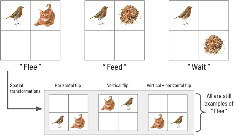
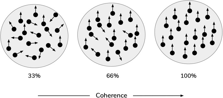
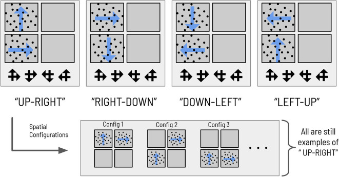
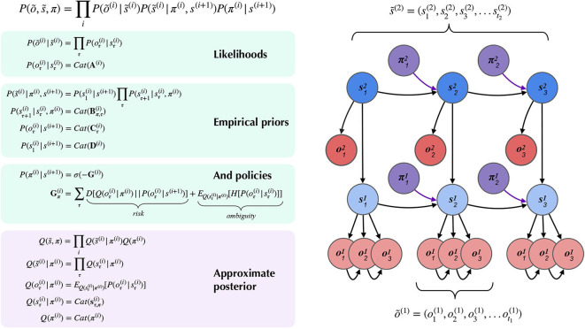
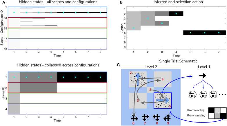
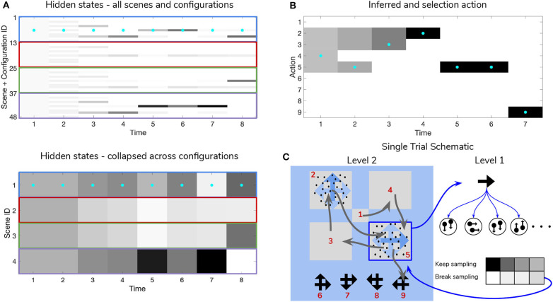
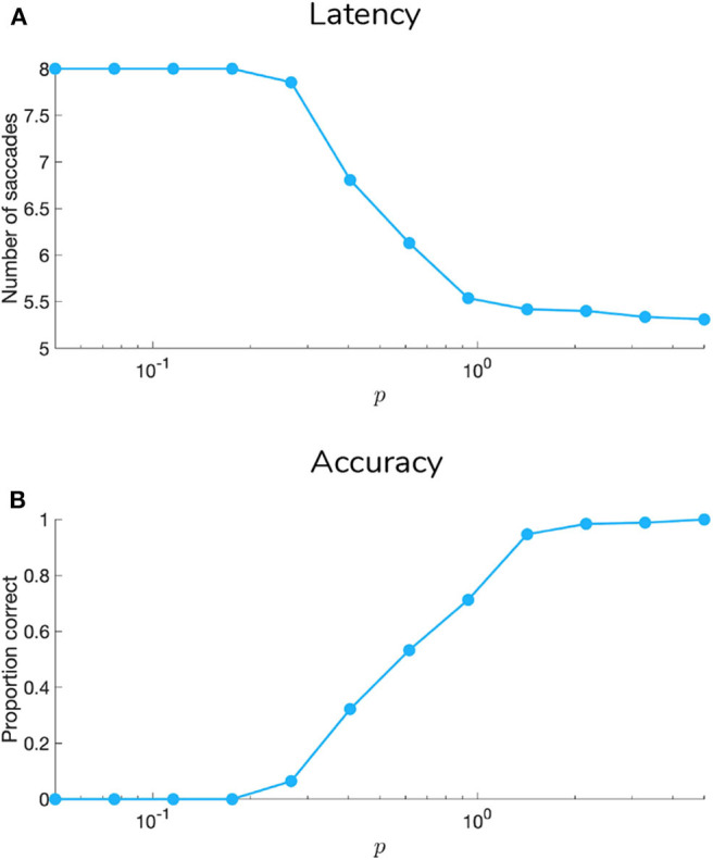
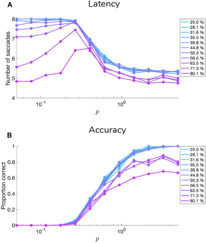
Adaptive agents must act in intrinsically uncertain environments with complex latent structure. Here, we elaborate a model of visual foraging-in a hierarchical context-wherein agents infer a higher-order visual pattern (a "scene") by sequentially sampling ambiguous cues. Inspired by previous models of scene construction-that cast perception and action as consequences of approximate Bayesian inference-we use active inference to simulate decisions of agents categorizing a scene in a hierarchically-structured setting. Under active inference, agents develop probabilistic beliefs about their environment, while actively sampling it to maximize the evidence for their internal generative model. This approximate evidence maximization (i.e., self-evidencing) comprises drives to both maximize rewards and resolve uncertainty about hidden states. This is realized via minimization of a free energy functional of posterior beliefs about both the world as well as the actions used to sample or perturb it, corresponding to perception and action, respectively. We show that active inference, in the context of hierarchical scene construction, gives rise to many empirical evidence accumulation phenomena, such as noise-sensitive reaction times and epistemic saccades. We explain these behaviors in terms of the principled drives that constitute the expected free energy, the key quantity for evaluating policies under active inference. In addition, we report novel behaviors exhibited by these active inference agents that furnish new predictions for research on evidence accumulation and perceptual decision-making. We discuss the implications of this hierarchical active inference scheme for tasks that require planned sequences of information-gathering actions to infer compositional latent structure (such as visual scene construction and sentence comprehension). This work sets the stage for future experiments to investigate active inference in relation to other formulations of evidence accumulation (e.g., drift-diffusion models) in tasks that require planning in uncertain environments with higher-order structure.

Keywords: Bayesian brain; active inference; epistemic value; free energy; hierarchical inference; random dot motion; visual foraging.

Figure 1

The scene configurations of the original formulation. The three scenes characterizing each trial in the original scene construction study, adapted with permission from Mirza et al. (2016).

Figure 2

Random Dot Motion Stimuli (RDMs). Schematic of random dot motion stimuli, with increasing coherence levels (i.e., % percentage of dots moving upwards) from left to right.

Figure 3

The mapping between scenes and RDMs. The mapping between the four abstract scene categories and their respective dot motion pattern manifestations in the context of the hierarchical scene construction task. As an example of the spatial invariance of each scene, the bottom right panels show two possible (out of 12 total) RDM configurations for the scene “RIGHT-DOWN,” where the two constitutive RDMs of that scene are found in exactly two of the four quadrants. The ‘scene symbols' at the bottom of the visual array represent the categorization choices available to the subject, with each symbol comprised of two overlapping arrows that indicate the directions of the motion that define the scene.

Figure 4

A partially-observed Markov Decision Process with two hierarchical layers. Schematic overview of the generative model for a hierarchical partially-observed Markov Decision Process. The generic forms of the likelihoods, priors, and posteriors at hierarchical levels are provided in the left panels, adapted with permission from Friston et al. (2017d). Cat(x) indicates a categorical distribution, and $\tilde{x}$ indicates a discrete sequence of states or random variables: $\tilde{x}=(x_1,x_2,\dots ,x_t)$. Note that priors at the highest level (Level 2) are not shown, but are unconditional (non-empirical) priors, and their particular forms for the scene construction task are described in the text. As shown in the “Empirical Priors” panel, prior preferences at lower levels ${\text{C}}_{\tau }^{(i)}$ can be a function of states at level i + 1, but this conditioning of preferences is not necessary, and in the current work we pre-determine prior preferences at lower levels, i.e., they are not contextualized by states at higher levels (see Figure 8). Posterior beliefs about policies are given by a softmax function of the expected free energy of policies at a given level. The approximate (variational) beliefs over hidden states are represented via a mean-field approximation of the full posterior, such that hidden states can be encoded as the product of marginal distributions. Factorization of the posterior is assumed across hierarchical layers, across hidden state factors (see the text and Figures 6, 7 for details on the meanings of different factors), and across time. “Observations” at the higher level (õ⁽²⁾) may belong to one of two types: (1) observations that directly parameterize hidden states at the lower level via the composition of the observation likelihood one level P(o^{(i + 1)}|s^{(i + 1)}) with the empirical prior or “link function” P(s⁽ⁱ⁾|o^{(i + 1)}) at the level below, and (2) observations that are directly sampled at the same level from the generative process (and accompanying likelihood of the generative model P(o^{(i + 1)}|s^{(i + 1)})). For conciseness, we represent the first type of mapping, from states at i + 1 to states at i through a direct dependency in the Bayesian graphical model in the right panel, but the reader should note that in practice this is achieved via the composition of two likelihoods: the observation likelihood at level i + 1 and the link function at level i. This composition is represented by a single empirical prior P(s⁽ⁱ⁾|s^{(i + 1)}) = Cat(D⁽ⁱ⁾) in the left panel. In contrast, all observations at the lowest level (õ⁽¹⁾) feed directly from the generative process to the agent.

Figure 5

Belief-updating under active inference. Overview of the update equations for posterior beliefs under active inference. (A) Shows the optimal solution for posterior beliefs about hidden states s^* that minimizes the variational free energy of observations. In practice the variational posterior over states is computed as a marginal message passing routine (Parr et al., 2019), where prediction errors ${\epsilon }_{\tau }^{\pi }$ minimized over time until some criterion of convergence is reached (ε ≈ 0). The prediction errors measure the difference between the current log posterior over states $ln{\text{s}}_{\tau }^{\pi }$ and the optimal solution ln s^*. Solving via error-minimization lends the scheme a degree of biological plausibility and is consistent with process theories of neural function like predictive coding (Bastos et al., ; Bogacz, 2017). An alternative scheme would be equating the marginal posterior over hidden states (for a given factor and/or timestep) to the optimal solution ${\text{s}}_{\pi ,\tau }^{*}$—this is achieved by solving for s^* when free energy is at its minimum (for a particular marginal), i.e., $\frac{\partial F}{\partial {\text{s}}_{\pi ,\tau }}=0$. This corresponds to a fixed-point minimization scheme (also known as coordinate-ascent iteration), where each conditional marginal is iteratively fixed to its free-energy minimum, while holding the remaining marginals constant (Blei et al., 2017). (B) Shows how posterior beliefs about policies are a function of the free energy of states expected under policies F and the expected free energy of policies G. F is a function of state prediction errors and expected states, and G is the expected free energy of observations under policies, shown here decomposed into the KL divergence between expected and preferred observations or risk (${\text{o}}_{\tau }^{\pi }·(ln{\text{o}}_{\tau }^{\pi }-{\text{C}}_{\tau })$) and the expected entropy or ambiguity ($\text{H}·{\text{s}}_{\tau }^{\pi }$). A precision parameter γ scales the expected free energy and serves as an inverse temperature parameter for a softmax normalization σ of policies. See the text (Section 4.1.1) for more clarification on the free energy of policies F. (C) Shows how actions are sampled from the posterior over policies, and the posterior over states is updated via a Bayesian model average, where expected states are averaged under beliefs about policies. Finally, expected observations are computed by passing expected states through the likelihood of the generative model. The right side shows a plausible correspondence between several key variables in an MDP generative model and known neuroanatomy. For simplicity, a hierarchical generative model is not shown here, but one can easily imagine a hierarchy of state inference that characterizes the recurrent message passing between lower-level occipital areas (e.g., primary visual cortex) through higher level visual cortical areas, and terminating in “high-level,” prospective and policy-conditioned state estimation in areas like the hippocampus. We note that it is an open empirical question, whether various computations required for active inference can be localized to different functional brain areas. This figure suggests a simple scheme that attributes different computations to segregated brain areas, based on their known function and neuroanatomy (e.g., computing the expected free energy of actions (G), speculated to occur in frontal areas).

Figure 6

Level 1 MDP. Level 1 of the hierarchical POMDP for scene construction (see Section 4.2.1 for details). Level 1 directly interfaces with stochastic motion observations generated by the environment. At this level hidden states correspond to: (1) the true motion direction s^(1),1 underlying visual observations at the currently-fixated region of the visual array and (2) the sampling state s^(1),2, an aspect of the environment that can be changed via actions, i.e., selections of the appropriate state transition, as encoded in the B matrix. The first hidden state factor s^(1),1 can either correspond to a state with no motion signal (“Null,” in the case when there is no RDM or a categorization decision is being made) or assume one of the four discrete values corresponding to the four cardinal motion directions. At each time step of the generative process, the current state of the RDM stimulus s^(1),1 is probabilistically mapped to a motion observation via the first-factor likelihood A^(1),1 (shown in the top panel as A_RDM). The entropy of the columns of this mapping can be used to parameterize the coherence of the RDM stimulus, such that the true motion states s^(1),1 cause motion observations o^(1),1 with varying degrees of fidelity. This is demonstrated by two exemplary A_{RDM state} matrices in the top panel (these correspond to A^(1),1): the left-most matrix shows a noiseless, “coherent” mapping, analogized to the situation of when an RDM consists of all dots moving in the same direction as described by the true hidden state; the matrix to the right of the noiseless mapping corresponds to an incoherent RDM, where instantaneous motion observations may assume directions different than the true motion direction state, with the frequency of this deviation encoded by probabilities stored in the corresponding column of A_RDM. The motion direction state doesn't change in the course of a trial (see the identity matrix shown in the top panel as B_RDM, which simply maps the hidden state to itself at each subsequent time step)—this is true of both the generative model and the generative process. The second hidden state factor s^(1),2 encodes the current “sampling state” of the agent; there are two levels under this factor: “Keep-sampling” or “Break-sampling.” This sampling state (a factor of the generative process) is directly represented as a control state in the generative model; namely, the agent can change it by sampling actions (B-matrix transitions) from the posterior beliefs about policies. The agent believes that the “Break-sampling” state is a sink in the transition dynamics, such that once it is entered, it cannot be exited (see the right-most matrix of the transition likelihood B_{Sampling state}). Entering the “Break-sampling” state terminates the POMDP at Level 1. The “Keep-sampling” state enables the continued generation of motion observations as samples from the likelihood mapping A^(1),1. A^(1),2 (the “proprioceptive” likelihood, not shown for clarity) deterministically maps the current sampling state s^(1),2 to an observation o^(1),2 thereof (bottom row of lower right panel), so that the agent always observes which sampling state it is in unambiguously.

Figure 7

Level 2 MDP. Level 2 of the hierarchical POMDP for scene construction. Hidden states consist of two factors, one encoding the scene identity and another encoding the eye position (i.e., current state of the oculomotor system). The first hidden state factor s^(2),1 encodes the scene identity of the trial in terms of two unique RDM directions occupy two of the quadrants (four possible scenes as described in the top right panel) and spatial configuration (one of 12 unique ways to place two RDMs in four quadrants). This yields a dimensionality of 48 for this hidden state factor (4 scenes × 12 spatial configurations). The second hidden state factor s^(2),2 encodes the eye position, which is initialized to be in the center of the quadrants (Location 1). The next four values of this factor index the four quadrants (2–5), and the last four are indices for the choice locations (the agent fixates one of these four options to guess the scene identity). As with the sampling state factor at Level 1, the eye position factor s^(2),2 is controllable by the agent through the action-dependent transition matrices B^(2),2. Outcomes at Level 2 are characterized by three modalities: the first modality o^(2),1 indicates the visual stimulus (or lack thereof) at the currently-fixated location. Note that during belief updating, the observations of this modality o^(2),1 are inferred hidden states over motion directions that are passed up after solving the Level 1 MDP (see Figure 6). An example likelihood matrix for this first modality is shown in the upper left, showing the conditional probabilities for visual outcomes when the 1st factor hidden state has the value 32. This corresponds to the scene identity DOWN-LEFT under spatial configuration 8 (the RDMs occupy quadrants indexed as Locations 2 and 4). The last two likelihood arrays A^(2),2 and A^(2),3 map to respective observation modalities o^(2),2 and o^(2),3, and are not shown for clarity; the A^(2),2 likelihood encodes the joint probability of particular types of trial feedback (Null, Correct, Incorrect—encoded by o^(2),2) as a function of the current hidden scene and the location of the agent's eyes, while A^(2),3 is an unambiguous proprioceptive mapping that signals to the agent the location of its own eyes via o^(2),3. Note that these two last observation modalities o^(2),2 and o^(2),3 are directly sampled from the environment, and are not passed up as “inferred observations” from Level 1.

Figure 8

C's and D's. Prior beliefs over observations and hidden states for both hierarchical levels. Note that superscripts here index the hierarchical level, and separate modalities/factors for the C and D matrices are indicated by stacked circles. At the highest level (Level 2), prior beliefs about second-modality outcomes (C^(2),2) encode the agent's beliefs about receiving correct and avoiding incorrect feedback. Prior beliefs over the other outcome modalities (C^(2),1 and C^(2),3) are all trivially zero. These beliefs are stationary over time and affect saccade selection at Level 2 via the expected free energy of policies G. Prior beliefs about hidden states D⁽²⁾ at this level encode the agent's initial beliefs about the scene identity and the location of their eyes. This prior over hidden states can be manipulated to put the agent's beliefs about the world at odds with the actual hidden state of the world. At Level 1, the agent's preferences about being in the “Break-sampling” state increases over time and is encoded in the preferences about second modality outcomes (C^(1),2), which corresponds to the agents umambiguous perception of its own sampling state. Finally, the prior beliefs about initial states at Level 1 (D¹) correspond to the motion direction hidden state (the RDM identity) as well as which sampling-state the agent is in. Crucially, the first factor of these prior beliefs D^(1),1 is initialized as the “expected observations” from Level 2: the expected motion direction (first modality). These expected observations are generated by passing the variational beliefs about the scene at Level 2 through the modality-specific likelihood mapping: Q(o^(2),1|s^(2),1) = P(o^(2),1|s^(2),1)Q(s^(2),1). The prior over hidden states at Level 1 is thus called an empirical prior as it is inherited from Level 2. The red arrow indicates the relationship between the expected observation from Level 2 and the empirical prior over (first-factor) hidden states at Level 1.

Figure 9

Simulated trial of scene construction under high sensory precision. (A) The evolution of posterior beliefs about scene identity—the first factor of hidden states at Level 2—as a deep active inference agent explores the visual array. In this case, sensory precision at Level 1 is high, meaning that posterior beliefs about the motion direction of each RDM-containing quadrant are resolved easily, resulting in fast and accurate scene categorization. Cells are gray-scale colored according to the probability of the belief for that hidden state and time index (darker colors correspond to higher probabilities). Cyan dots indicates the true hidden state at each time step. The top row of (A) shows evolving beliefs about the fully-enumerated scene identity (48 possibilities), with every 12 configurations highlighted with a differently-colored bounding box, correspond to beliefs about each type of scene (i.e., UP-RIGHT, RIGHT-DOWN, DOWN-LEFT, LEFT-UP). The bottom panel shows the collapsed beliefs over the four scenes, computed by summing the hidden state beliefs across the 12 spatial configurations. (B) Evolution of posterior beliefs about actions (fixation starting location not shown), culminating in the categorization decision (here, the scene was categorized as UP-RIGHT, corresponding to a saccade to location 6. (C) Visual representation of the agent's behavior for this trial. Saccades are depicted as curved gray lines connecting one saccade endpoint to the next. Fixation locations (corresponding to 2nd factor hidden state indices) are shown as red numbers. The Level 1 active inference process occurring within a single fixation is schematically represented on the right side, with individual motion samples shown as issued from the true motion direction via the low level likelihood A^(1),1. The agent observes the true RDM at Level 1 and updates its posterior beliefs about this hidden state. As uncertainty about the RDM direction is resolved, the “Break-sampling” action becomes more attractive (since epistemic value contributes increasingly less to the expected free energy of policies). In this case, the sampling process at Level 1 is terminated after only three timesteps, since the precision of the likelihood mapping is high (p = 5.0) which relates to the speed at which uncertainty is resolved about the RDM motion direction—see the text for more details.

Figure 10

Simulated trial of scene construction with low sensory precision. Same as in Figure 9, except in this trial the precision of the mapping between RDM motion directions and samples thereof is lower, p = 0.5. This leads to an incorrect sequence of inferences, where the agent ends up believing that the scene identity is LEFT-UP and guessing incorrectly. Note that after this choice is made and incorrect feedback is given, the agent updates their posterior in terms of the “next best” guess, which is from the agent's perspective either UP-RIGHT or DOWN-LEFT (see the posterior at Time step 8 of (A)). (C) Shows that the relative imprecision of the Level 1 likelihood results in a sequence of stochastic motion observations that frequently diverge from the true motion direction (in this case, the true motion direction is RIGHT in the lower right quadrant (Location 5)). Level 1 belief-updating gives rise to an imprecise posterior belief over motion directions that are passed up as inferred outcomes to Level 2, leading to false beliefs about the scene identity. Note the “ambivalent,” quadrant-revisiting behavior, wherein the agent repeatedly visits the lower-right quadrant to resolve uncertainty about the RDM stimulus at that quadrant.

Figure 11

Effect of sensory precision on scene construction performance. Average categorization latency (A) and accuracy (B) as a function of sensory precision p which controls the entropy of the (Level 1) likelihood mapping from motion direction to motion observation. We simulated 185 trials of scene construction under hierarchical active inference for each level of p (12 levels total), with scene identities and configurations randomly initialized for each trial. Sensory precision is shown on a logarithmic scale.

Figure 12

Effect of sensory precision on scene construction performance for different prior belief strengths. Same as in Figure 11 but for different strengths of initial prior beliefs (legend on right). Prior belief strengths are defined as the probability density of the prior beliefs about hidden states (1st hidden state factor of Level 2—D^(2),1) concentrated upon one of the four possible scenes. This elevated probability is uniformly spread among the 12 hidden states corresponding to the different quadrant-configurations of that scene, such that the agent has no prior expectation about a particular arrangement of the scene, but rather about that scene type in general. Here, we only show the results for agents with “incorrect” prior beliefs—namely, when the scene that the agent believes to be at play is different from the scene actually characterizing the trial.

Figure 13

Effect of sensory precision on quadrant dwell time. (A) Shows the effect of increasing sensory precision at Level 1 on the time it takes to switch to “Break-sampling” policy. Here, 250 trials were simulated for each combination of sensory precision and prior belief strength, with priors over hidden states at Level 2 randomly initialized to have high probability about 1 of the 4 scene types. Break-times were analyzed only for the first saccade (at Level 2) of each trial. (B) Shows the effect of sensory precision on evolution of the relative posterior probabilities of the “Keep-sampling” vs. the “Break-sampling” policies (Policy Differential = P_{Keep-sampling}−P_{Break-sampling}). We only show these posterior policy differentials for the first 10 time steps of sampling at Level 1 due to insufficient numbers of saccades that lasted more than 10 time steps at the highest/lowest sensory precisions (see A). Averages are calculated across different prior belief strengths, based on the lack of an effect, as is apparent in (A). The policy differential defined in this way is always positive because as soon as the probability of “Break-sampling” exceeds that of “Keep-sampling” (i.e., Policy Differential < 0), the “Break-sampling” policy will be engaged with near certainty. This is due the high precision over policies at the lower level (here, γ = 512), which essentially ensures that the policy with higher probability will always be selected.

References

1. Bastos A., Usrey W., Adams R., Mangun G., Fries P., Friston K. (2012). Canonical microcircuits for predictive coding. Neuron 76, 695–711. 10.1016/j.neuron.2012.10.038 - DOI - PMC - PubMed
1. Beal M. J. (2004). Variational algorithms for approximate bayesian inference (Ph.D. thesis), Gatsby Unit, University College London, London, United Kingdom.
1. Biehl M., Guckelsberger C., Salge C., Smith S. C., Polani D. (2018). Expanding the active inference landscape: more intrinsic motivations in the perception-action loop. Front. Neurorobot. 12:45. 10.3389/fnbot.2018.00045 - DOI - PMC - PubMed
1. Blei D. M., Kucukelbir A., McAuliffe J. D. (2017). Variational inference: a review for statisticians. J. Am. Stat. Assoc. 112, 859–877. 10.1080/01621459.2017.1285773 - DOI
1. Bogacz R. (2017). A tutorial on the free-energy framework for modelling perception and learning. J. Math. Psychol. 76, 198–211. 10.1016/j.jmp.2015.11.003 - DOI - PMC - PubMed