Bound2Learn: a machine learning approach for classification of DNA-bound proteins from single-molecule tracking experiments

Abstract

DNA-bound proteins are essential elements for the maintenance, regulation, and use of the genome. The time they spend bound to DNA provides useful information on their stability within protein complexes and insight into the understanding of biological processes. Single-particle tracking allows for direct visualization of protein-DNA kinetics, however, identifying whether a molecule is bound to DNA can be non-trivial. Further complications arise when tracking molecules for extended durations in processes with slow kinetics. We developed a machine learning approach, termed Bound2Learn, using output from a widely used tracking software, to robustly classify tracks in order to accurately estimate residence times. We validated our approach in silico, and in live-cell data from Escherichia coli and Saccharomyces cerevisiae. Our method has the potential for broad utility and is applicable to other organisms.

Figure 1.

Approach to isolate DNA-bound molecules. (A) Diagram of experimental setup to do single-molecule tracking with photoactivatable/photoconvertible fluorophores to calculate residence times on DNA. (B) Variables from Trackmate used to predict if a track represents a genuine bound molecule. (C) Illustration of the general procedure for ML and how it can be used to predict tracks from experimental data for POI. (D) Top: Example images from simulations of single-molecule movies representing E. coli cells and budding yeast nuclei. Bottom: Illustration of the variables used in ML models 1 and 2. (E) Example of plot to help tune hyperparameters to minimize OOB error. (F) Test data results for different ML models.

Figure 2.

Estimating residence times over a range of conditions. (A) Top: Diagram illustrating the GMM fit to determine the mean of mean speed for 1 s interval data, which can be used to rescale the speed variables. Bottom – Estimates of residence times in both simulations (n = 169 tracks for E. coli and n = 232 tracks for budding yeast). (B) Distribution of apparent diffusion coefficients from E. coli simulation, with GMM fitting, followed by clustering to isolate tracks representing bound molecules (blue) and diffusing/noise (orange). n = 291 tracks. (C) Top: Diagram illustrating the GMM fit to maximum quality values from a data set with lower fluorescent intensities. Bottom: Estimates of residence times from simulated data representing poorer image quality (n = 159 tracks for E. coli and n = 227 tracks for budding yeast). (D) Top: Example of image from simulated 100 ms timelapse in E. coli. (E) Two-exponential fitting to a data set with heterogeneous population of bound molecules (n = 508 tracks). For all estimates, 95% confidence intervals are shown.

Figure 3.

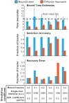
Testing Bound2Learn under challenging simulation conditions for tracking. Simulations were done based on E. coli cells and the same tracking analysis parameters were used across all conditions. The input bound time was 8 s while the bleach time was 20 s. Images represented 500 ms exposure with a 1 s time interval. Error bars for bound time estimates represent 95% confidence intervals.

Figure 4.

Estimating residence times for PolIII subunit, ϵ. (A) Example of ϵ-mMaple timelapse. Red circles indicate molecules that were classified as being bound with Bound2Learn. Scale bar = 2 μm. (B) Histogram and fit of track durations from combined data set of ϵ. (C) Estimation of residence times and comparison to estimates from (1). Estimate for β was a weighted average calculated from bound times estimated with different time intervals. (D) Summary of results showing both mean track duration estimates and mean bound time estimates from combined data sets. 95% confidence intervals are shown next to estimates.

Figure 5.

Estimating residence time of Top2 and TBP in budding yeast. (A) Example of Top2-HaloTag timelapse after photoactivation. Yellow circle indicates molecule classified as being bound with Bound2Learn. Cell and nucleus outlines are drawn in white and cyan, respectively. Also shown is the SME of a Pol30-mNeonGreen z-stack. Scale bar = 3 μm. (B) Violin plots of track durations for Top2 (n = 94), and Histone H3 (n = 123). Error bars represent 95% confidence intervals. Dotted horizontal lines represent upper and lower bounds of the 95% confidence interval of Histone H3. (C) Histogram and fit on Top2 track durations. Note that bin counts for short durations are smaller than expect given that short tracks of <4 localizations were discarded. This was compensated for during the fitting procedure (Materials and Methods). Errors are represented by 95% confidence intervals (D) Example of SPT15-HaloTag (TBP) timelapse collected with continuous exposure, after photoactivation. Yellow circles indicate molecules classified as being bound by Bound2Learn. Cell and nucleus outlines are drawn in white and cyan, respectively. Also shown is the SME of a Pol30-mNeonGreen z-stack. Scale bar = 3 μm. (E) Violin plots of track durations for TBP (n = 729), and Histone H3 (n = 242). Error bars represent 95% confidence intervals. Dotted horizontal lines represent upper and lower bounds of the 95% confidence interval of Histone H3. (F) Histogram and fit on TBP track durations, along with estimate for bound time. (G) Estimates for diffusive properties and static localization errors of ML classified bound tracks, obtained through fitting averaged MSD curves. (H) Summary of results showing both mean track duration estimates and mean bound time estimates from combined data sets. 95% confidence intervals are shown next to estimates.

References

1. Beattie T.R., Kapadia N., Nicolas E., Uphoff S., Wollman A.J.M., Leake M.C., Reyes-Lamothe R.. Frequent exchange of the DNA polymerase during bacterial chromosome replication. Elife. 2017; 6:e21763. - PMC - PubMed
1. Uphoff S., Reyes-Lamothe R., de Leon F.G., Sherratt D.J., Kapanidis A.N.. Single-molecule DNA repair in live bacteria. Proc. Natl. Acad. Sci. U.S.A. 2013; 110:8063–8068. - PMC - PubMed
1. Mazza D., Abernathy A., Golob N., Morisaki T., McNally J.G.. A benchmark for chromatin binding measurements in live cells. Nucleic Acids Res. 2012; 40:e119. - PMC - PubMed
1. Hager G.L., McNally J.G., Misteli T.. Transcription dynamics. Mol. Cell. 2009; 35:741–753. - PMC - PubMed
1. Mehta G.D., Ball D.A., Eriksson P.R., Chereji R.V., Clark D.J., McNally J.G., Karpova T.S.. Single-molecule analysis reveals linked cycles of RSC chromatin remodeling and Ace1p transcription factor binding in yeast. Mol. Cell. 2018; 72:875–887. - PMC - PubMed
Publication types
Grants and funding