Model-based analysis and forecast of sleep-wake regulatory dynamics: Tools and applications to data

Abstract

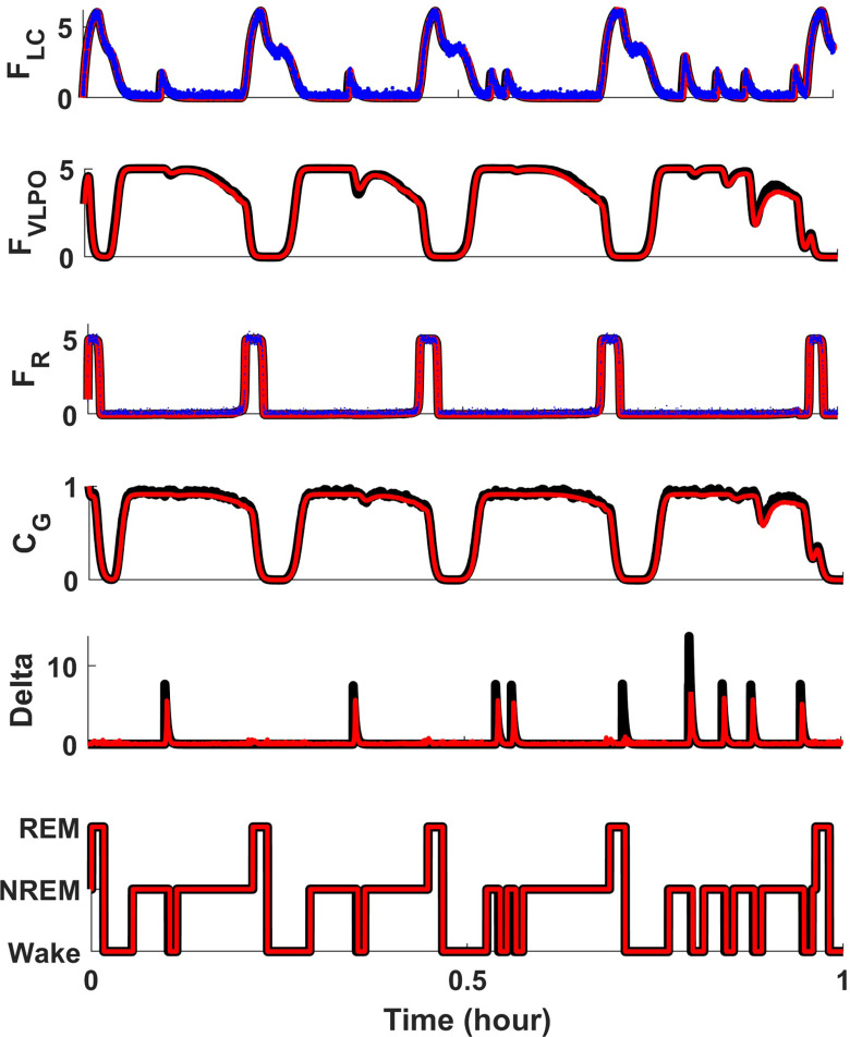
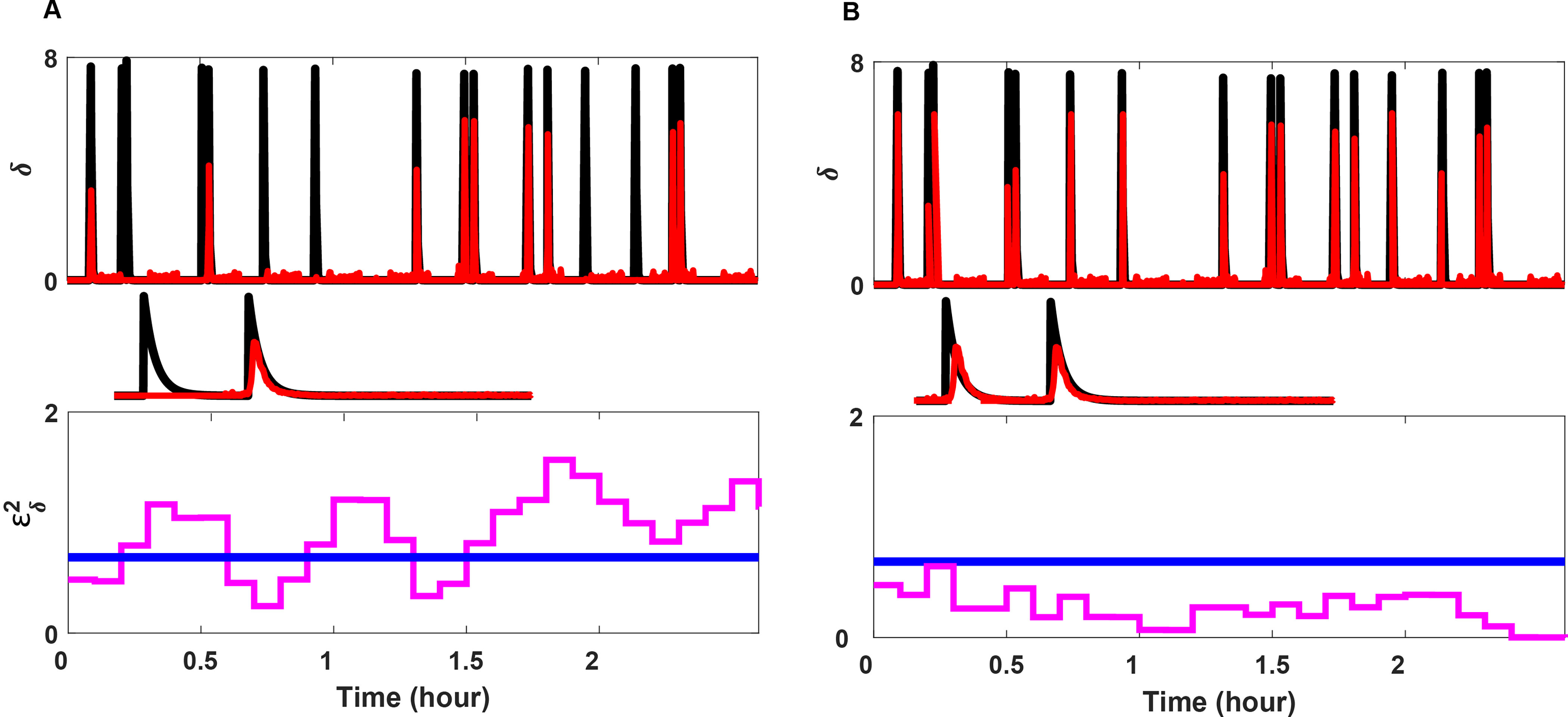
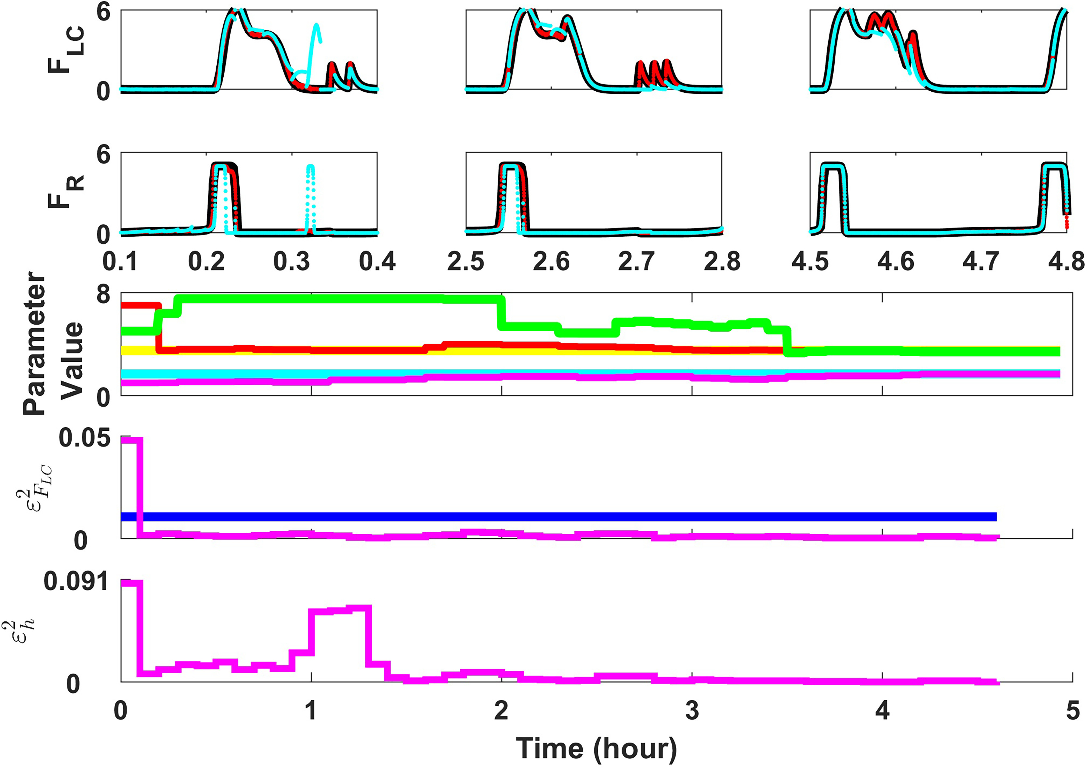
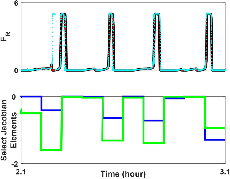
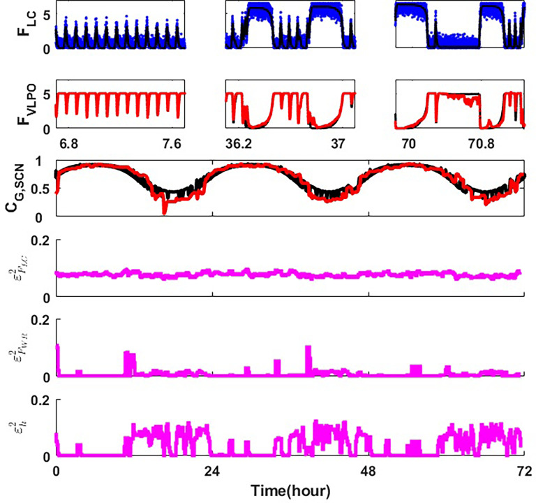
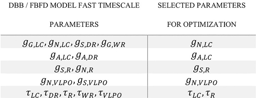
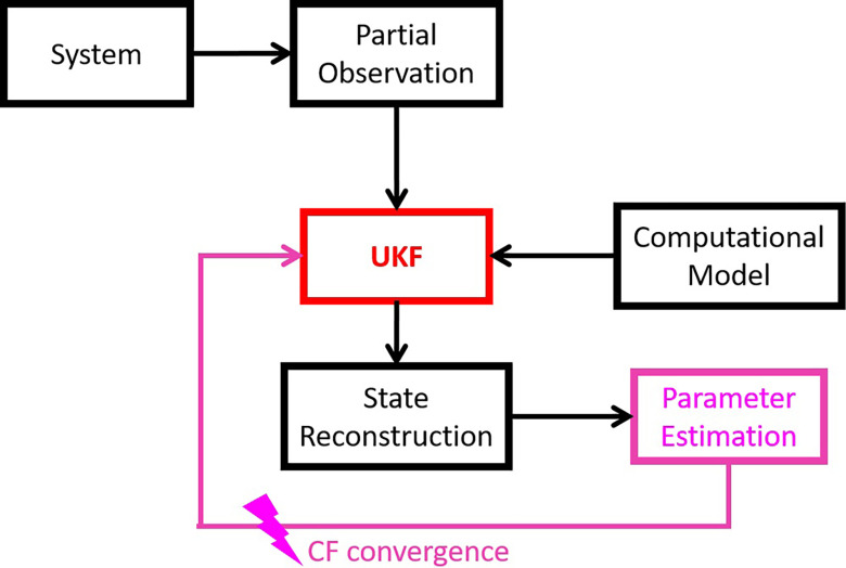
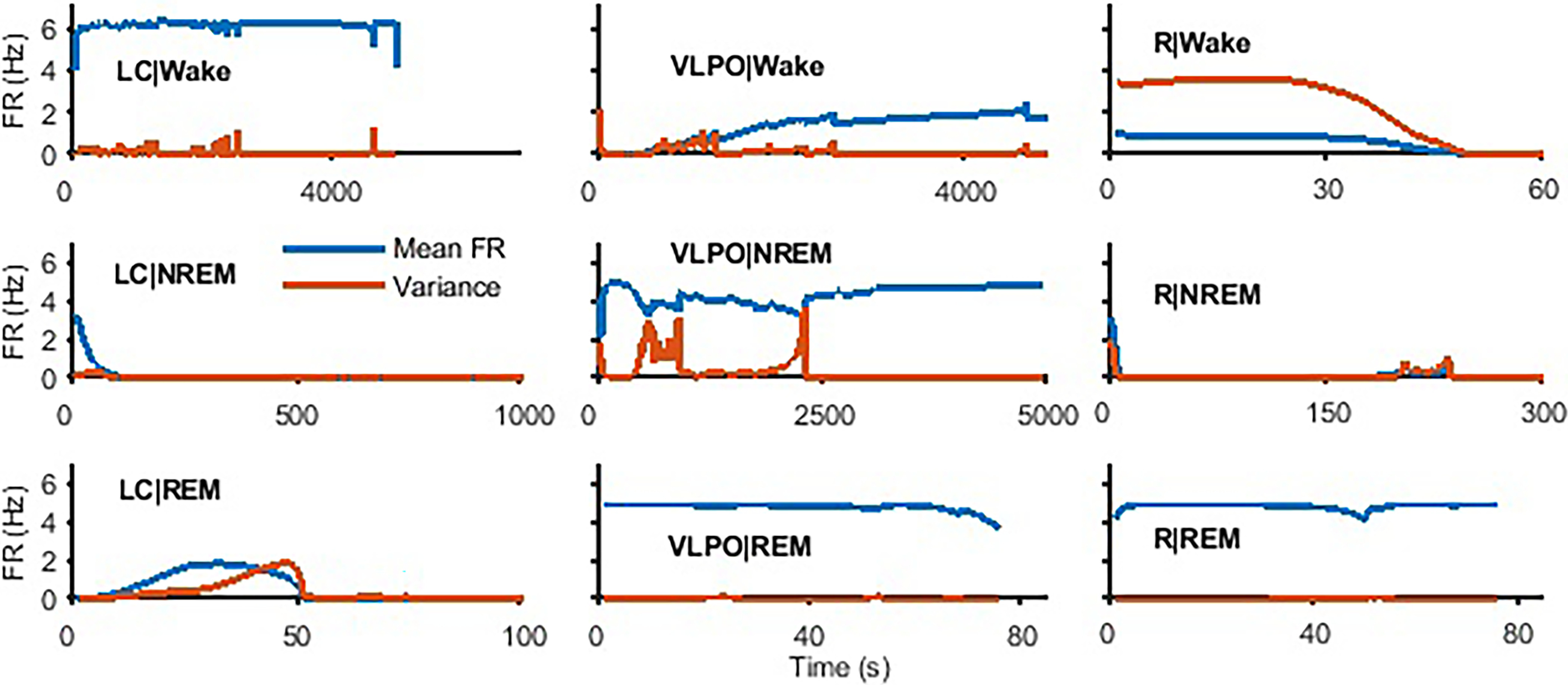
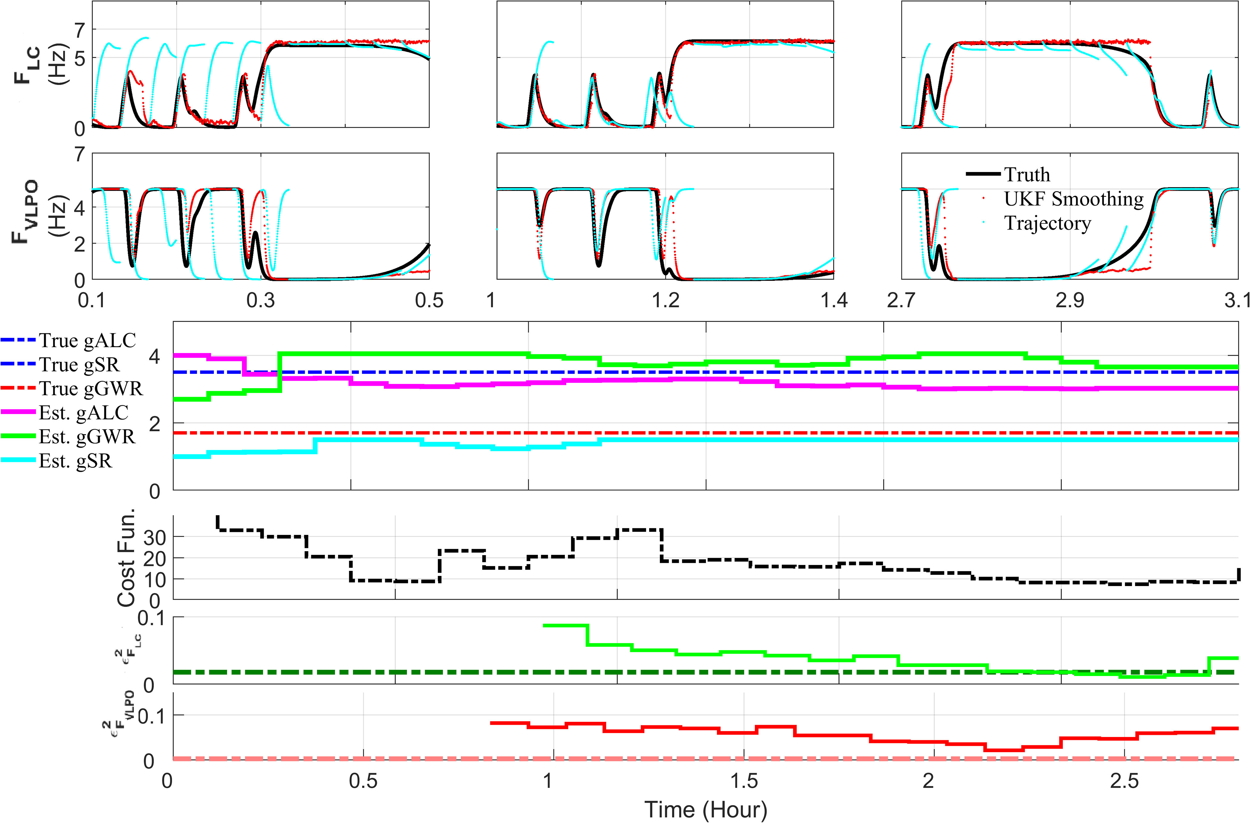
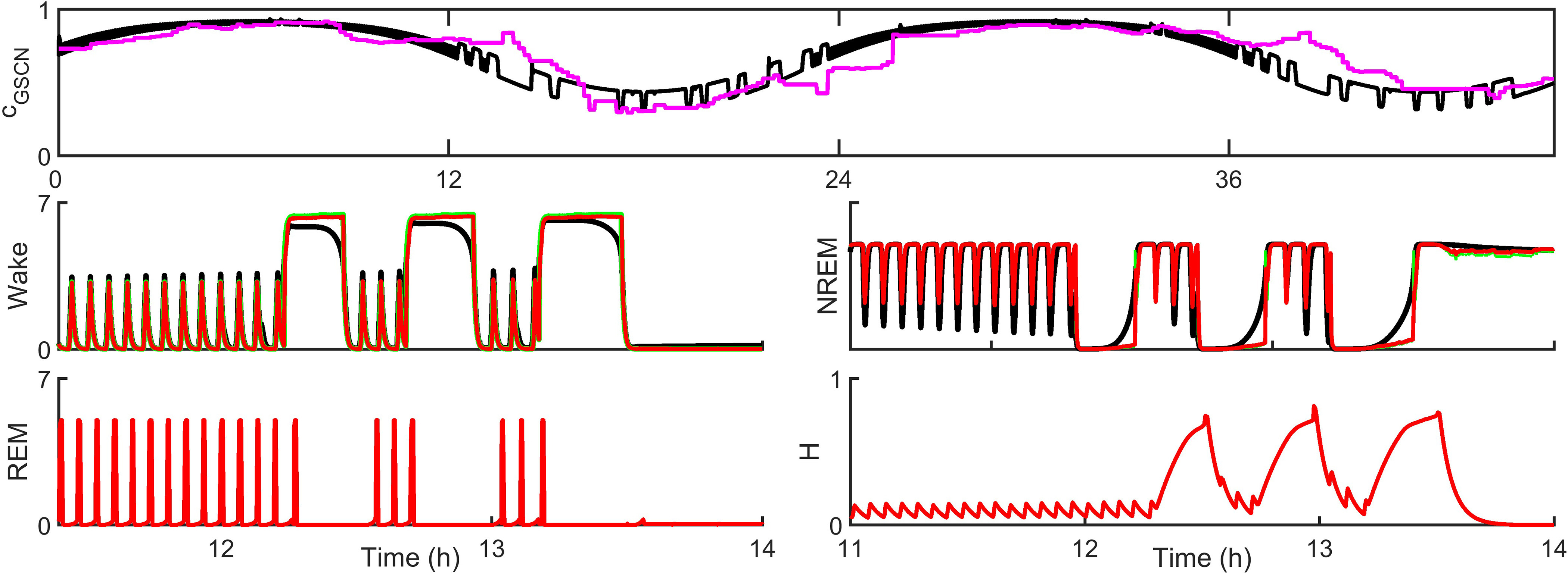
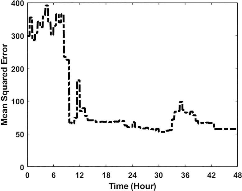
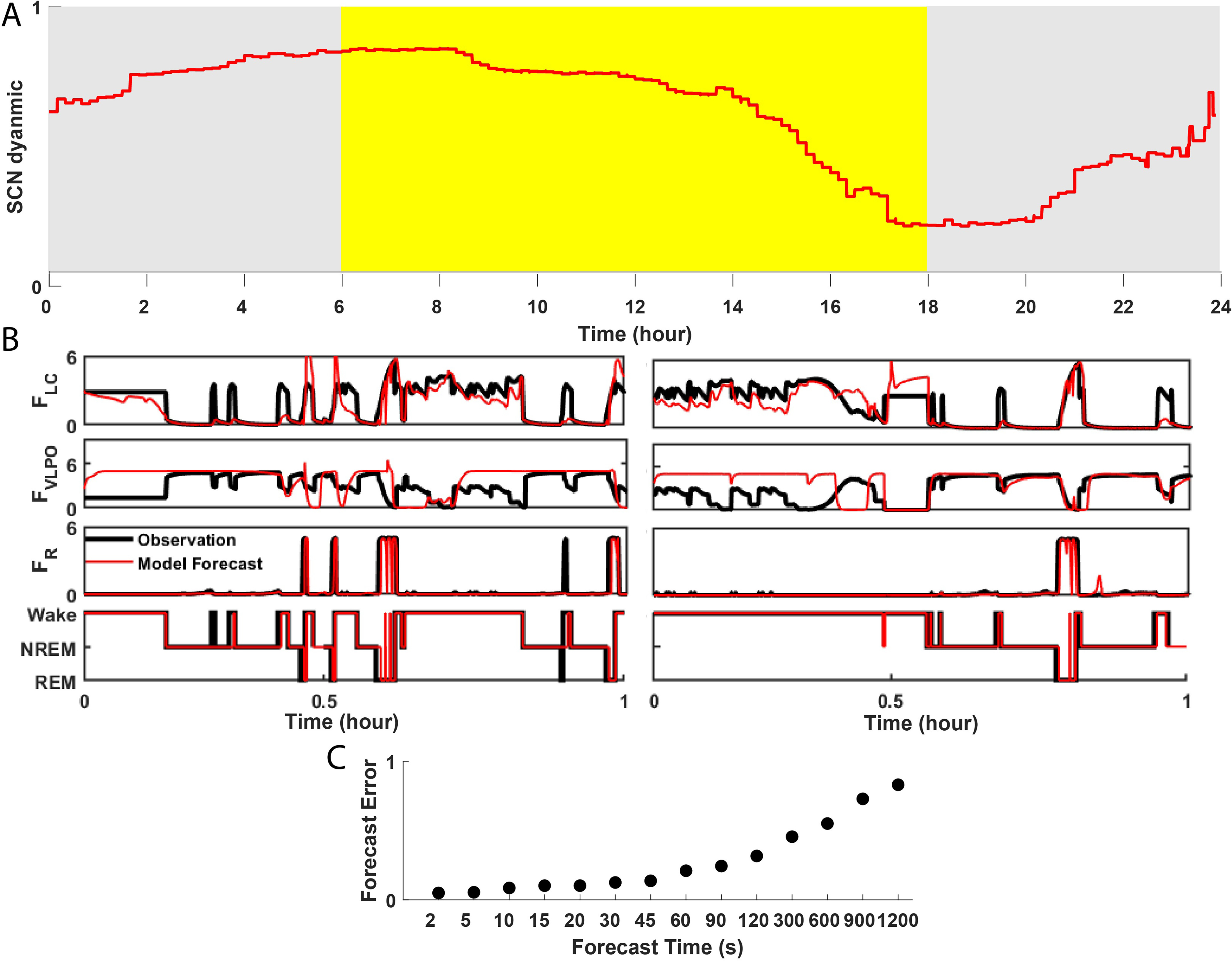
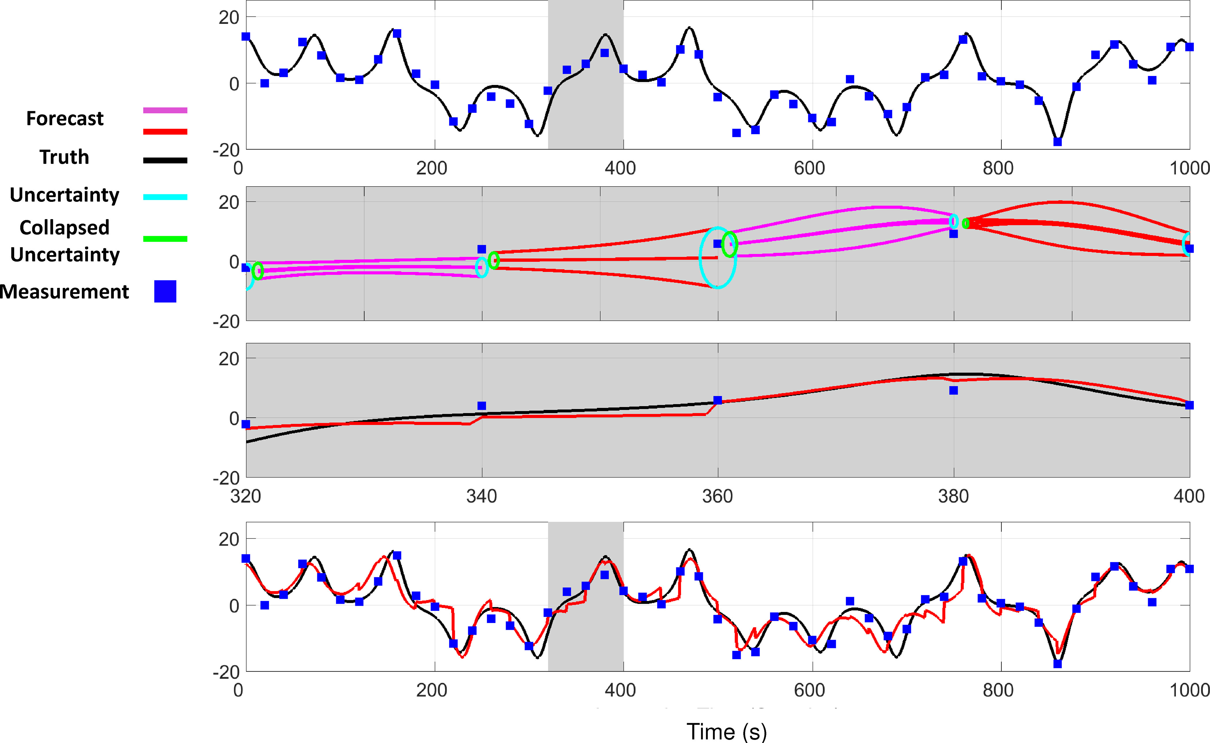
Extensive clinical and experimental evidence links sleep-wake regulation and state of vigilance (SOV) to neurological disorders including schizophrenia and epilepsy. To understand the bidirectional coupling between disease severity and sleep disturbances, we need to investigate the underlying neurophysiological interactions of the sleep-wake regulatory system (SWRS) in normal and pathological brains. We utilized unscented Kalman filter based data assimilation (DA) and physiologically based mathematical models of a sleep-wake regulatory network synchronized with experimental measurements to reconstruct and predict the state of SWRS in chronically implanted animals. Critical to applying this technique to real biological systems is the need to estimate the underlying model parameters. We have developed an estimation method capable of simultaneously fitting and tracking multiple model parameters to optimize the reconstructed system state. We add to this fixed-lag smoothing to improve reconstruction of random input to the system and those that have a delayed effect on the observed dynamics. To demonstrate application of our DA framework, we have experimentally recorded brain activity from freely behaving rodents and classified discrete SOV continuously for many-day long recordings. These discretized observations were then used as the "noisy observables" in the implemented framework to estimate time-dependent model parameters and then to forecast future state and state transitions from out-of-sample recordings.

FIG. 1.

Example of DBB model dynamics and UKF reconstruction. Shown are ODE-integrated state dynamics (black traces) and reconstructed state (red traces). State variables shown are firing rates for the wake-active (LC: $F_{LC}$), NREM-active ($F_{VLPO}$ ), and REM-active (LDT/PPT: $F_R$) cell groups, neurotransmitter GABA concentration ($C_G$), thalamic noise ($\delta$), as well as the hypnogram. Noise-contaminated measurements of $F_{LC}$ and $F_R$ (blue) were passed to the unscented Kalman filter (UKF) framework to reconstruct all other state variables. Here, the framework was given, and the parameter values were used to generate data and random initial conditions. The reconstructed firing rate dynamics (red) quickly approach and track the true (black) dynamics. The stochastically driven $\delta$ dynamics are only somewhat reconstructed.

FIG. 2.

Effect of smoothing on reconstruction accuracy of $\delta$. (a) Default values of the model with no smoother result in poor reconstruction of $\delta$ even with optimized values for CI. The black trace represents the original model-generated data as ground truth. The reconstructed $\delta$ with optimized CI is shown in red. (b) Using a smoother will reduce the reconstruction error of $\delta$ to less than half its original reconstruction metric (blue trace).The reconstructed, smoothed $\delta$ with optimized CI is shown in red. The insets in A and B show the dynamics of reconstructed $\delta$ using smoothing expanded within the 0.5-0.6 time-range.

FIG. 3.

Parameter estimation with the LM method. We chose three different parameters: $g_{S,R}$, $g_{A,LC}$, and $g_{G,WR}$ for fitting while observing F${}_{LC}$ and F${}_R$. Parameter estimation is performed using a multiple-shooting method: the divergence of short model-generated trajectories that originate on the reconstructed trajectories from the UKF-reconstructed dynamics is minimized. This divergence minimization is done over time windows longer than the cycle time of the dynamics to better sample the state space. Here, we use 20-min long windows, with a 6-min overlap. The trajectories for the short model generated (cyan), reconstructed (red), and true (black) F${}_{LC}$ and F${}_R$ dynamics for different periods of the convergence of the three parameters are shown in the first two panels. We start with random initial values for each parameter and estimate its correct value at each step: $g_{S,R}$ (green), $g_{A,LC}$ (red), and $g_{G,WR}$ (magenta). Yellow and cyan traces indicate the correct value of the parameters. For parameter values significantly different than the true value, the short trajectories diverge quickly from the reconstructed values, which in turn results in a poorly reconstructed state. As parameters approach their true values, both short model-generated and reconstructed trajectories approach their true values as well. Reconstruction metric ${ϵ}_i^2$ is computed for each data assimilation window for all variables. Here, in the last two panels, the reconstruction metric for the original noisy observation of F${}_{LC}$ as well as an unobserved variable h is shown. The reconstruction metric for both F${}_{LC}$ and h decreases as the parameters converge to their correct values. Note that parameter estimation has the effect of optimizing unmeasured state reconstruction.

FIG. 4.

Changes in the Jacobian of the cost function with respect to $g_{S,R}$ during REM transitions. The true firing rate of the REM-active cell group (F${}_R$) is indicated by the black trace. The cyan and red traces indicate the model-generated trajectories and UKF reconstruction, respectively. The parameters $g_{S,R}$ and $g_{A,LC}$ are chosen for fitting. As F${}_R$ peaks, $\frac{\mathrm{\partial }(CF)}{\mathrm{\partial }(g_{S,R})}$ (green trace), which is a directly REM-coupled parameter, increases. However, the $\frac{\mathrm{\partial }(CF)}{\mathrm{\partial }(g_{A,LC})}$ trace (blue) directly linked to the wake cell group LC does not change. The change in Jacobian marks the parameters that are going to change given where in the dynamical state the trajectories are. This will reduce unnecessary computational burden to fit all parameters at all times.

FIG. 5.

Parameter estimation for tracking of circadian dynamics. Noisy measurements of F${}_{LC}$ from the full FBFD model were assimilated with a version of the DBB model that represented input from the SCN as a quasi-static parameter $C_{G,SCN}$ whose value was estimated and tracked in overlapping 30-min long windows (6 minute overlap). Two upper panel: Short excerpts of reconstructed dynamics for various phases of the circadian cycle are shown for F${}_{LC}$ and F${}_{VLPO}$ where black, blue, and red traces indicate true model values, the observation, and the UKF reconstruction, respectively. Third panel: Estimated (red) and true (black) value of the tracked parameter $C_{G,SCN}$ are shown. Note that the tracked parameter value is estimated with inherent smoothing on the timescale of a 30 min and does not reconstruct the feedback of the sleep–wake regulatory cell groups to the SCN. Normalized reconstruction error for various variables is shown in the lower three panels. The reconstruction of unobserved variables F${}_{WR}$ and homeostatic sleep drive h is quite good as indicated by small ${ϵ}^2$ values.

FIG. 6.

Optimized fast timescale parameters. We used a subset of data with relatively constant SCN dynamics to estimate fast timescale parameters. Based on parameter correlation calculations, described in Sec. III C 2, a subset of these parameters were optimized. Parameters included in the steady state firing rate function, $VLP{O}_{max}$, $L{C}_{max}$, $D{R}_{max}$, $R_{max}$, $W{R}_{max}$, $\alpha$, and $\beta$ values were fixed using the original model values. The parameters determine relative maximum firing rates of each cell group and are not significantly modulated by sleep dynamics.

FIG. 7.

Procedural steps of the DA-UKF algorithm. The data assimilation framework receives the observed data, whether noisy model-generated data or experimental SOV, makes forecasts, corrects its predicted SOV trajectory and model parameters according to observed data, and then repeats the process.

FIG. 8.

Hypnogram derived observations for the FBFD model dynamics. Mean (blue traces) and variance (red traces) for $F_{LC}$, $F_{VLPO}$, and $F_R$ from model-generated data as a function of time from state transitions into identified SOV. Because state and time since last transition can be causally measured from hypnograms, we use these means and variances as inferred observation functions to translate hypnogram into state- and state-transition conditioned observations.

FIG. 9.

Hypnogram derived simultaneous state tracking and multiple parameter fitting. We chose three different parameters: g${}_{S,R}$, g${}_{A,LC}$, and g${}_{G,WR}$ for fitting while observing F${}_{LC}$, F${}_{VLPO}$, and F${}_R$ derived from the hypnogram. Parameter estimation is performed with the multiple-shooting method described in Sec. III C 3 over 20-min long windows, with a 6-min overlap. The trajectories for the short model generated (cyan), reconstructed (red), and true (black) F${}_{LC}$ and F${}_{VLPO}$ dynamics for different periods of the convergence of the three parameters are shown in the first two panels. We start with random initial values for each parameter and estimate its correct value at each step: g${}_{S,R}$ (cyan), g${}_{A,LC}$ (magenta), and g${}_{G,WR}$ (green). Dashed lines indicate the correct value of the parameters. Note that initially, for parameter values significantly different from the true value, the short trajectories diverge quickly from the reconstructed values, and the reconstructed values of F${}_{LC}$ and F${}_{VLPO}$ are different from the true values. When the parameters approach their true values, both short model-generated and reconstructed trajectories approach their true values as well and the cost function (CF) approaches zero (black trace). Reconstruction metric ${ϵ}_i^2$ is computed for each data assimilation window and is shown in the last two panels for F${}_{LC}$ (green) and F${}_{VLPO}$ (red). As a reference, the variance of the noisy observations of F${}_{LC}$ and F${}_{VLPO}$ is also shown in dashed green and red lines. ${ϵ}_i^2$ decreases as the parameters and states approach their correct values.

FIG. 10.

Hypnogram derived simultaneous state tracking and multiple parameter fitting for SCN. The observations are the hypnogram derived F${}_{LC}$ and F${}_{VLPO}$. After estimating the fast parameters with a constant SCN, we utilized the estimated parameter values to estimate SCN over longer time-periods. The estimated $C_{G,SCN}$ (magenta) follows the true value relatively well (black). This results in good reconstruction of the other model variables such as the firing rate during REM (indicated by REM) and the homeostatic sleep drive (H). Observation of F${}_{LC}$ (Wake) and F${}_{VLPO}$ (NREM) are indicated by green traces.

FIG. 11.

Reconstruction results using DA-UKF and experimental SOV from rodents. The model predictions are corrected at every measurement point. The cost function, similar to Fig. 9, is calculated as the difference between original model values and the ones derived from animal SOV. The model predictions converge and seem to stabilize after about 12 h.

FIG. 12.

Reconstruction and forecast of SCN and SOV from animal data. (a) SCN dynamics were predicted within the DA-UKF framework with experimentally measured animal SOV. The SCN was reconstructed and averaged over 5 days to form a 24-h long time-series. The yellow and gray backgrounds indicate the animal day and night, respectively. (b) Model forecast for out-of-sample data is shown in red for 1 h in the animal’s day when the animal mostly sleeps (left panel) and for 1 h in the animal’s night when the animals are mostly awake (right panel). The original experimental SOV and firing rate traces derived from the SOV are shown in black. The firing rates shown are $F_{LC}$ from wake-active LC, $F_{VLPO}$ from NREM-active VLPO, and $F_R$ from REM-active PPT/LDT cell groups. The model is set to forecast every 5 s with a fixed update rate of 5 s. (c) Forecast error (FE) as a function of forecast time. FE was computed as the mean value of the binary test that the forecast SOV equaled the experimentally measured SOV. FE was computed for 24 h of out of sample data. FE increases as the forecast horizon becomes longer.

FIG. 13.

Unscented Kalman Filter (UKF) algorithm and output. UKF uses a prediction–correction scheme, where the predictions come from the mathematical equations that govern the model, given to the UKF, and the correction comes from measurements. UKF starts with a set of initial conditions that it propagates through the model equations and builds a set of forecast trajectories (shown in red). This process will continue until a measurement point. At that point, the UKF compares the forecast trajectories with the measurement value. Based on the error, it either widens or tightens the cloud of points and builds the next set of forecast trajectories (magenta). As time goes on, the error in the trajectories diverges unless they are corrected based on the measurements.

References

1. Wulff K., Gatti S., Wettstein J. G., and Foster R. G., “Sleep and circadian rhythm disruption in psychiatric and neurodegenerative disease,” Nat. Rev. Neurosci. 11, 589–599 (2010). 10.1038/nrn2868 - DOI - PubMed
1. Pritchett D., Wulff K., Oliver P. L., Bannerman D. M., Davies K. E., Harrison P. J., Peirson S. N., and Foster R. G., “Evaluating the links between schizophrenia and sleep and circadian rhythm disruption,” J. Neural Transm. 119, 1061–1075 (2012). 10.1007/s00702-012-0817-8 - DOI - PubMed
1. Sedigh-Sarvestani M., Schiff S. J., and Gluckman B. J., “Reconstructing mammalian sleep dynamics with data assimilation,” PLoS Comput. Biol. 8, 1002788 (2012). 10.1371/journal.pcbi.1002788 - DOI - PMC - PubMed
1. Datta S. and MacLean R. R., “Neurobiological mechanisms for the regulation of mammalian sleep-wake behavior: Reinterpretation of historical evidence and inclusion of contemporary cellular and molecular evidence,” Neurosci. Biobehav. Rev. 31, 775–824 (2007). 10.1016/j.neubiorev.2007.02.004 - DOI - PMC - PubMed
1. Saper C. B., Scammell T. E., and Lu J., “Hypothalamic regulation of sleep and circadian rhythms,” Nature 437, 1257–1263 (2005). 10.1038/nature04284 - DOI - PubMed
LinkOut - more resources