Improving reconstructive surgery design using Gaussian process surrogates to capture material behavior uncertainty

Abstract

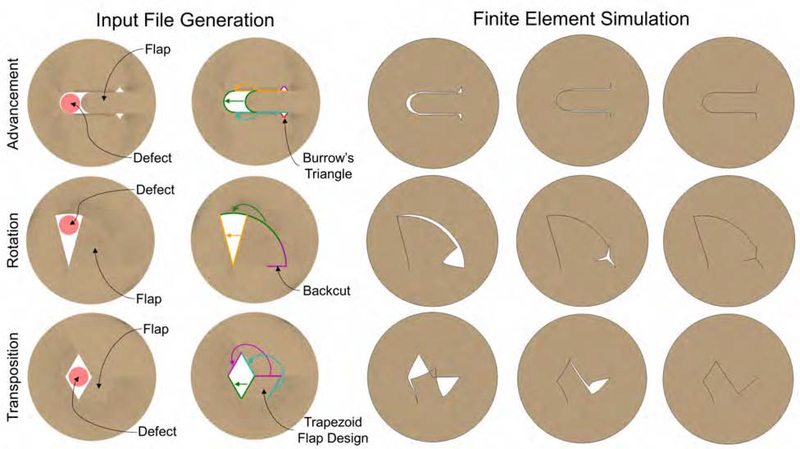
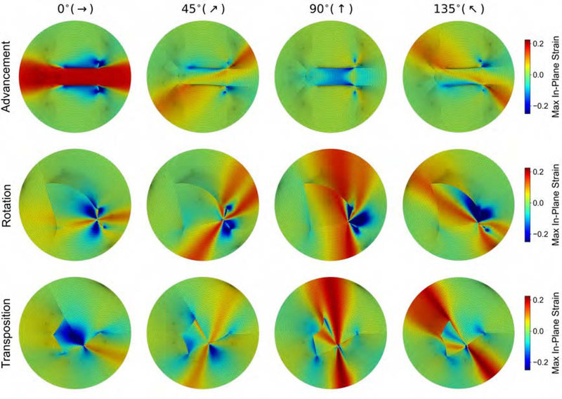
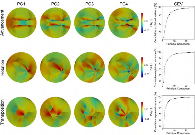
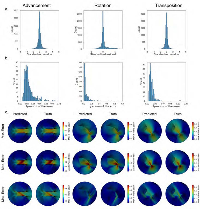
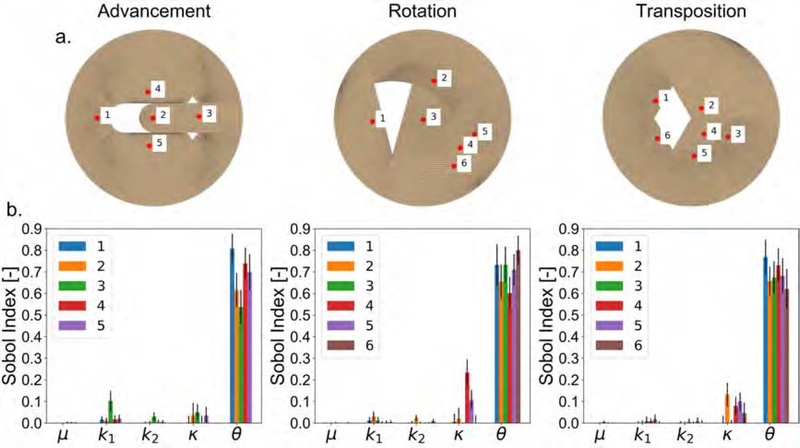
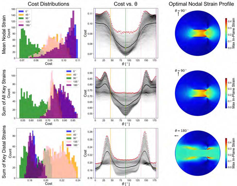
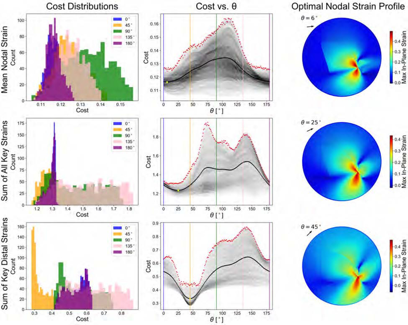
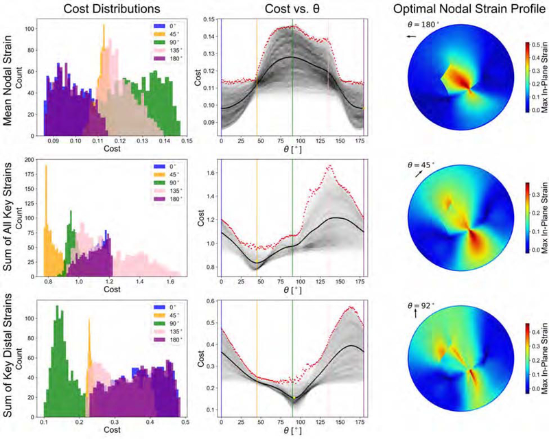
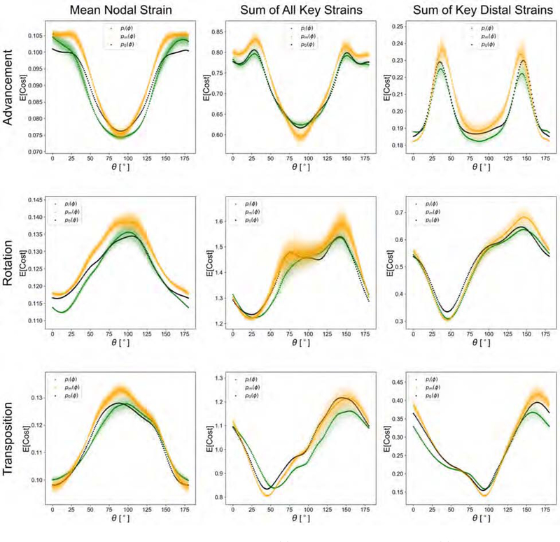
To produce functional, aesthetically natural results, reconstructive surgeries must be planned to minimize stress as excessive loads near wounds have been shown to produce pathological scarring and other complications (Gurtner et al., 2011). Presently, stress cannot easily be measured in the operating room. Consequently, surgeons rely on intuition and experience (Paul et al., 2016; Buchanan et al., 2016). Predictive computational tools are ideal candidates for surgery planning. Finite element (FE) simulations have shown promise in predicting stress fields on large skin patches and in complex cases, helping to identify potential regions of complication. Unfortunately, these simulations are computationally expensive and deterministic (Lee et al., 2018a). However, running a few, well selected FE simulations allows us to create Gaussian process (GP) surrogate models of local cutaneous flaps that are computationally efficient and able to predict stress and strain for arbitrary material parameters. Here, we create GP surrogates for the advancement, rotation, and transposition flaps. We then use the predictive capability of these surrogates to perform a global sensitivity analysis, ultimately showing that fiber direction has the most significant impact on strain field variations. We then perform an optimization to determine the optimal fiber direction for each flap for three different objectives driven by clinical guidelines (Leedy et al., 2005; Rohrer and Bhatia, 2005). While material properties are not controlled by the surgeon and are actually a source of uncertainty, the surgeon can in fact control the orientation of the flap with respect to the skin's relaxed tension lines, which are associated with the underlying fiber orientation (Borges, 1984). Therefore, fiber direction is the only material parameter that can be optimized clinically. The optimization task relies on the efficiency of the GP surrogates to calculate the expected cost of different strategies when the uncertainty of other material parameters is included. We propose optimal flap orientations for the three cost functions and that can help in reducing stress resulting from the surgery and ultimately reduce complications associated with excessive mechanical loading near wounds.

Keywords: Local flaps; Machine learning; Nonlinear finite elements; Skin biomechanics; Soft tissue mechanics.

Figure 1:

Skin is a multilayered tissue composed of three layers: epidermis, dermis, hypodermis. The epidermis is an approximately 50 − 200μm thick stratified epithelial tissue made out of keratinocytes. The dermis is 1–4 mm in thickness, is the main load bearing layer of the skin due to its high collagen content. The hypermis is the bottom layer, made out of adipose tissue. The interface between the skin and the underlying muscle is the fascia. Cutaneous flaps such as advancement, rotation and transposition flaps involve undermining of the tissue, i.e. detachment of the skin from the underlying fascia.

Figure 2:

The three most common flap designs are advancement, rotation and transposition flaps. FE models of the flaps are generated semi-automatically. The Base flap design is generated manually in Abaqus. Identification of the edges is done automatically. Matching colored edges in each design are brought together by sutures to close the skin as indicated by the arrows. Adjacent skin regions to the edges are also identified and used to impose essential boundary conditions. In this case, only the outer perimeter is fixed. Suturing pattern imposed as linear constraints between pairs of nodes are applied gradually to bring the flap together. In this case, the sutures are mapped across the paired edges such that they have a uniform spacing. Snapshots of the simulation are shown, depicting how the edges are brought together as it would be done in the surgical setting. For the advancement flap, the skin of the flap is directly moved into the space previously occupied by the defect, with removal of Burrow’s triangles at the base of the flap. For the rotation flap, the skin flap describes an arc of rotation toward the regions previously occupied by the defect, with a proximal back-cut allowing suturing of the proximal end. In the transposition flap, a trapezoid is designed in the proximal tissues and transposed to fill the defect.

Figure 3:

The distribution of maximum in-plane strain for the advancement, transposition, and rotation flaps at θ = [0°, 45°, 90°, 135°] with all other parameters set to the mean values of their range. The maximum in plane strain in the figure is based on the maximum absolute value. Strain patterns show features spanning the entire skin region and aligning with the fiber orientation.

Figure 4:

First 4 PCs plotted on the finite element meshes for each of the three flaps. Cumulative explained variance (CEV) in accounting for 99% of the variation in the total data is shown in the last column for each of the flaps. The first 4 PCs explain 86.1%, 85.3%, and 88.5% of the advancement, rotation and transposition flaps respectively. PCs form an alternative basis for the strain profiles which enable compressing of the data into very few features compared to the number of nodes. Ultimately, to account for 99% of the variance, 26 PCs were kept as a truncated basis for the advancement case, 24 for the rotation, and 23 for the transposition flap.

Figure 5:

a) Standardized residuals computed from comparing surrogate predictions and validation data after it has been projected onto the PC basis. b) L2 Norm of the relative error between the surrogate and the validation data. To obtain strains, the predictions of the PC scores from the individual GP surrogates are transformed via inverse PCA to the strain space. c) surrogate predictions versus FE truth for the minimum, median, and maximum L2 norm relative errors.

Figure 6:

a) Locations of key points used in the sensitivity analysis and in the optimization steps. b) Sobol index for the nodal strain at each of the key points after completing the analysis using 12,000 predictions from the surrogate model.

Figure 7:

Results of optimization for the advancement flap. The first column shows cost distributions for five values of θ. The second column shows the cost versus θ plots. The vertical lines of different color correspond to the selected values of θ in the first column. In the middle column, the shaded area corresponds to the distribution of the cost as samples from p₀(ϕ) are taken. The expected value of the cost is shown as the black solid line, and the minimum of this expectation is the yellow point in the plot. The red data points show the worst case scenario computed from the particle swarm optimization for each θ. The strain profile corresponding to the minimum expected cost is shown in the third column. The rows denote the three different cost functions introduced in the main text

Figure 8:

Results of optimization for the rotation flap. The first column shows cost distributions for five values of θ. The second column shows the cost versus θ. The vertical lines correspond to the selected values of θ in the first column. The shaded area shows the distribution of the cost obtained from sampling values from p₀(ϕ), the prior over the material parameters. The solid black line is the expected cost with minimum indicated by the yellow point. The red data points show the worst case scenario obtained from the particle swarm optimizer for each value of θ. The strain profile corresponding to the minimum expected cost is shown in the third column. Each row corresponds to a different cost function.

Figure 9:

Results of optimization for the transposition flap. The first column shows cost distributions for five values of θ. The second column shows the cost versus θ. The vertical lines of different color correspond to the selected values of θ in the first column. The solid black line in the middle column is the curve of the expected cost as a function of θ, while the gray shaded regions show the distribution of the cost which follows from sampling material parameters from p₀(ϕ).The yellow points on the expected cost curve denotes the minimum of the curve. The worst case scenario for each θ obtained with the particle swarm optimizer is depicted with red points on the middle column. The strain profile corresponding to the minimum expected cost is shown in the third column.

Figure 10:

Expected value of cost for 3 distributions of the material parameters p(ϕ): entire range, uniform distribution (p₀(ϕ)); mean of range, normal distribution (p_m(ϕ)); and 59 year old female, normal distribution (p_i(ϕ)). The shaded regions around p_m(ϕ) and p_i(ϕ) indicate the cost distribution, while the solid line denotes the expectation of the cost. For the prior distribution p₀(ϕ) only the expected cost is shown.

References

-
- Gurtner GC, Dauskardt RH, Wong VW, Bhatt KA, Wu K, Vial IN, Padois K, Korman JM, Longaker MT, Improving cutaneous scar formation by controlling the mechanical environment: large animal and phase i studies, Annals of surgery 254 (2011) 217–225. - PubMed
- Buchanan PJ, Kung TA, Cederna PS, Evidence-based medicine: wound closure, Plastic and reconstructive surgery 138 (2016) 257S–270S. - PubMed
- Lee T, Turin SY, Gosain AK, Bilionis I, Tepole AB, Propagation of material behavior uncertainty in a nonlinear finite element model of reconstructive surgery, Biomechanics and modeling in mechanobiology 17 (2018) 1857–1873. - PubMed
- Leedy JE, Janis JE, Rohrich RJ, Reconstruction of acquired scalp defects: an algorithmic approach, Plastic and reconstructive surgery 116 (2005) 54e–72e. - PubMed
Publication types
MeSH terms
Grants and funding
LinkOut - more resources
Full Text Sources
Other Literature Sources