Reconstructing feedback representations in the ventral visual pathway with a generative adversarial autoencoder

Abstract

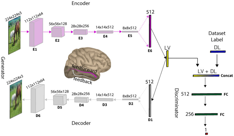
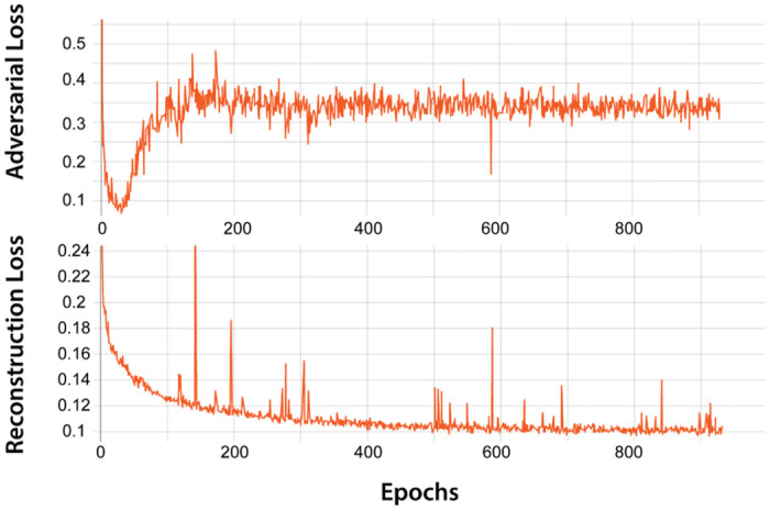
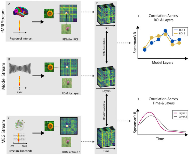
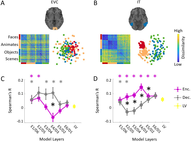
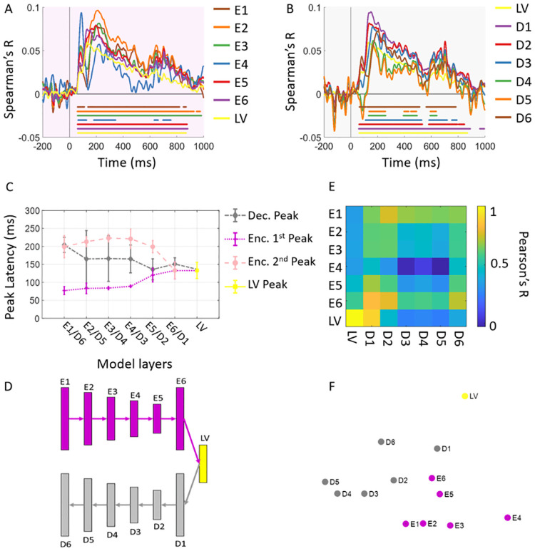
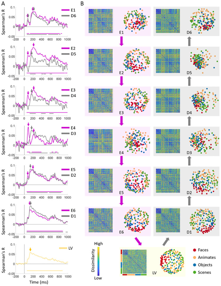
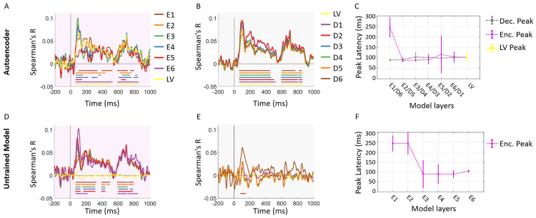
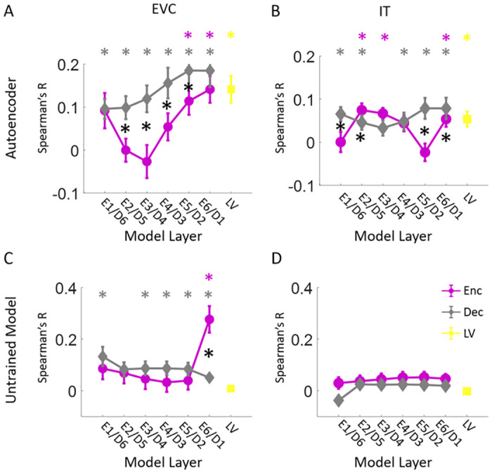
While vision evokes a dense network of feedforward and feedback neural processes in the brain, visual processes are primarily modeled with feedforward hierarchical neural networks, leaving the computational role of feedback processes poorly understood. Here, we developed a generative autoencoder neural network model and adversarially trained it on a categorically diverse data set of images. We hypothesized that the feedback processes in the ventral visual pathway can be represented by reconstruction of the visual information performed by the generative model. We compared representational similarity of the activity patterns in the proposed model with temporal (magnetoencephalography) and spatial (functional magnetic resonance imaging) visual brain responses. The proposed generative model identified two segregated neural dynamics in the visual brain. A temporal hierarchy of processes transforming low level visual information into high level semantics in the feedforward sweep, and a temporally later dynamics of inverse processes reconstructing low level visual information from a high level latent representation in the feedback sweep. Our results append to previous studies on neural feedback processes by presenting a new insight into the algorithmic function and the information carried by the feedback processes in the ventral visual pathway.

Fig 1. Computational model architecture.

The model is a generative adverserial network. The generator is an autoencoder consisting of five convolutional blocks (E1-E5) and one fully connected layer (E6) in the encoder and one fully connected layer (D1) followed by five deconvolutional blocks in the decoder (D2-D6). Each convolutional block encompasses batch normalization, convolution, nonlinear activation function (Leaky Rectified Linear Unit), and pooling operations. Alternatively, each deconvolutional block encompasses batch normalization, transposed convolution, nonlinear activation function (Leaky Rectified Linear Unit), and upsampling operations. The discriminator consists of two fully connected layers. The training Data set consists of 1,980,000 images organized into four super-ordinate categories: (i) Faces, (ii) Animates, (iii) Objects, (iv) Scenes. LV denotes the latent vector generated by the encoder and DL is a one-hot data set label (one of the four mentioned training data sets). Both vectors are concatenated and fed to the discriminator, while only the latent vector is fed to the decoder.

Fig 2. Computational model performance.

(A) Adversarial and Reconstruction loss over training epochs.

Fig 3. Representational similarity analysis to compare fMRI, MEG and model representations.

(A) fMRI response patterns were extracted from each ROI and pairwise condition-specific dissimilarities (1-Pearson’s R) were computed to create one fMRI RDM per ROI and participant (see Materials and methods section for detail). (B) RDMs for the generative model were computed at each convolutional/deconvolutional block after feeding 156 images to the computational model. (C) MEG data consists of time-series data with 306 channels and 1200 time points (milliseconds) per trial. For each condition, we extracted a vector of size 306 at each time point as the whole brain activity pattern to compute the RDMs using SVM classifiers decoding accuracies (see Materials and methods section for detail). (D) Using RDMs from MEG and fMRI ROIs, we compared (Spearman’s R) them with the RDMs from the computational model to investigate the spatio-temporal correspondences between the human brain and the computational model. (E) Correlations between ROI fMRI RDMs and computational model RDMs result in a subject-specific correlation value for each ROI across model layers, which we then average them over subjects. (F) Correlations between time-resolved MEG RDMs and computational model RDMs result in a subject-specific signal for each layer across time, which we then average them over subjects.

Fig 4. Spatial representational comparisons.

(A) Neural representations in early visual cortex (EVC). The subject-averaged EVC RDM matrix, and its 2D multidimensional scaling visualization. (B) Neural representations in inferior temporal area (IT). The subject-averaged IT RDM matrix, and its 2D multidimensional scaling visualization. (C) Encoder, decoder and LV layer RDMs are correlated (Spearman’s R) with subject-specific EVC RDMs. The averaged correlations over subjects with standard error of the mean are depicted. (D) Encoder, decoder and LV layer RDMs are correlated (Spearman’s R) with subject-specific IT RDMs. The averaged correlations over subjects with standard error of the mean are depicted. The color coded (*) above each panel in C-D indicates that the correlation of the corresponding layer is significantly above zero. The black (*) indicates the correlations of the corresponding encoder and decoder layers are significantly different (N = 15; two-sided ttests; false discovery rate corrected at P < 0.05).

Fig 5. Temporal representational comparisons.

(A) Encoder and MEG representational comparison. We correlated the encoder layer RDMs with subject-specific time-resolved MEG RDMs resulting in fifteen correlation time courses. We then averaged these time courses over participants. (B) Decoder and MEG representational comparison. Correlation of the decoder layer RDMs and time-resolved MEG RDMs. The color-coded lines below the curves show the time points when the correlations are significantly above zero (N = 15; permutation tests; cluster definition threshold P < 0.01; cluster threshold P < 0.05). (C) Peak latency for encoder and decoder. The encoder have significantly earlier peak latency across all layers (P = 0.014). Error bars are expressed in standard error of the mean. (D) The architecture of the models with layers’s label corresponding to (C). (E) The visualization of relationships between model layers representations. The matrix of RDM correlations between encoder and decoder layers is depicted. Each matrix entry compares two RDMs indexed by corresponding row and column in terms of Pearson’s R. (F) The multidimensional scaling visualization of the RDMs relationships.

Fig 6. Comparisons of encoder and decoder representational dynamics.

(A) Comparison of correlation time series of the encoder and decoder layers with the same level of processing. The color-coded lines below the curves show the timepoints when the correlations are significantly above zero (N = 15; permutation tests; cluster definition threshold P < 0.01; cluster threshold P < 0.05). (B) The model RDMs and their corresponding MDS visualizations.

Fig 7. The impact of architecture and training procedure on the representational similarity of the model and brain temporal data.

(A) Comparison of the encoder layers of the autoencoder model with MEG representations. We correlated the encoder layer RDMs with subject-specific time-resolved MEG RDMs resulting in fifteen correlation time courses. We then averaged these time courses over participants. (B) Comparison of the decoder layers of the autoencoder model with MEG representations. Correlation of the decoder layer RDMs and time-resolved MEG RDMs. The color-coded lines below the curves show the time points when the correlations are significantly above zero (N = 15; permutation tests; cluster definition threshold P < 0.01; cluster threshold P < 0.05). (C) Peak latency for encoder and decoder of the autoencoder model. Error bars are expressed in standard error of the mean. (D) Comparison of the encoder layers of the untrained model with MEG representations. We correlated the encoder layer RDMs with subject-specific time-resolved MEG RDMs resulting in fifteen correlation time courses. We then averaged these time courses over participants. (E) Comparison of the decoder layers of the untrained model with MEG representations. Correlation of the decoder layer RDMs and time-resolved MEG RDMs. The color-coded lines below the curves show the time points when the correlations are significantly above zero (N = 15; permutation tests; cluster definition threshold P < 0.01; cluster threshold P < 0.05). (F) Peak latency for encoder and decoder of the untrained model. Error bars are expressed in standard error of the mean.

Fig 8. The impact of architecture and training procedure on the representational similarity of the model and brain spatial data.

(A) Encoder, decoder and LV layer RDMs of the autoencoder model are correlated (Spearman’s R) with subject-specific EVC RDMs. The averaged correlations over subjects with standard error of the mean are depicted. (B) Encoder, decoder and LV layer RDMs of the autoencoder model are correlated (Spearman’s R) with subject-specific IT RDMs. The averaged correlations over subjects with standard error of the mean are depicted. (C) Encoder, decoder and LV layer RDMs of the untrained model are correlated (Spearman’s R) with subject-specific EVC RDMs. The averaged correlations over subjects with standard error of the mean are depicted. (D) Encoder, decoder and LV layer RDMs of the untrained model are correlated (Spearman’s R) with subject-specific IT RDMs. The averaged correlations over subjects with standard error of the mean are depicted. The color coded (*) above each panel in C-D indicates that the correlation of the corresponding layer is significantly above zero. The black (*) indicates the correlations of the corresponding encoder and decoder layers are significantly different (N = 15; two-sided ttests; false discovery rate corrected at P < 0.05).

References

1. Epstein R, Kanwisher N. A cortical representation the local visual environment. Nature. 1998;392(6676):598–601. 10.1038/33402 - DOI - PubMed
1. Epstein R, Harris A, Stanley D, Kanwisher N. The parahippocampal place area: Recognition, navigation, or encoding? Neuron. 1999;23(1):115–125. 10.1016/S0896-6273(00)80758-8 - DOI - PubMed
1. Cichy RM, Khosla A, Pantazis D, Oliva A. Dynamics of scene representations in the human brain revealed by magnetoencephalography and deep neural networks. NeuroImage. 2017;153:346–358. 10.1016/j.neuroimage.2016.03.063 - DOI - PMC - PubMed
1. Lowe MX, Rajsic J, Ferber S, Walther DB. Discriminating scene categories from brain activity within 100 milliseconds. Cortex. 2018;106:275–287. 10.1016/j.cortex.2018.06.006 - DOI - PubMed
1. Henriksson L, Mur M, Kriegeskorte N. Rapid invariant encoding of scene layout in human OPA. Neuron. 2019;103(1):161–171. 10.1016/j.neuron.2019.04.014 - DOI - PubMed
Publication types
LinkOut - more resources