Blood Flow Velocimetry in a Microchannel During Coagulation Using Particle Image Velocimetry and Wavelet-Based Optical Flow Velocimetry

Abstract

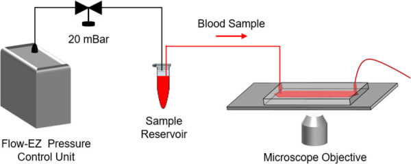
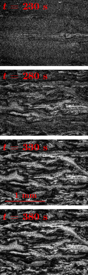
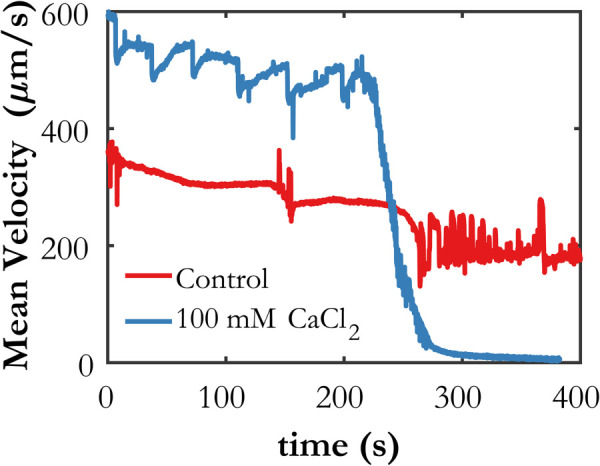
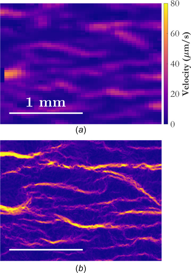
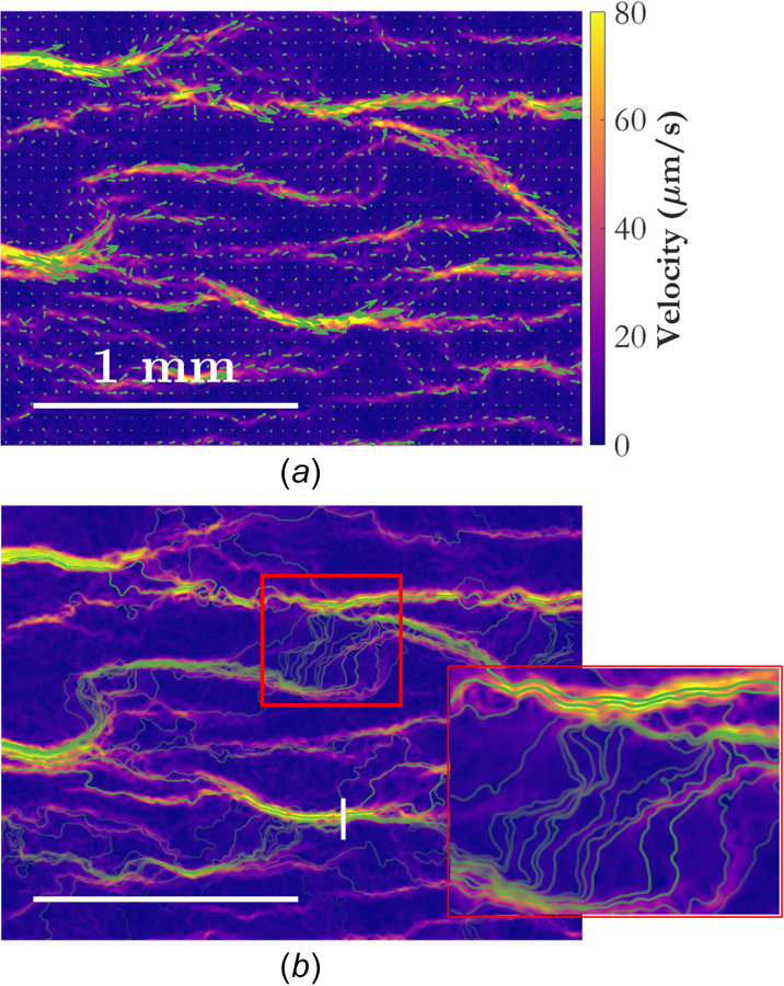
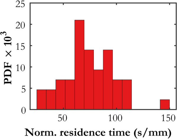
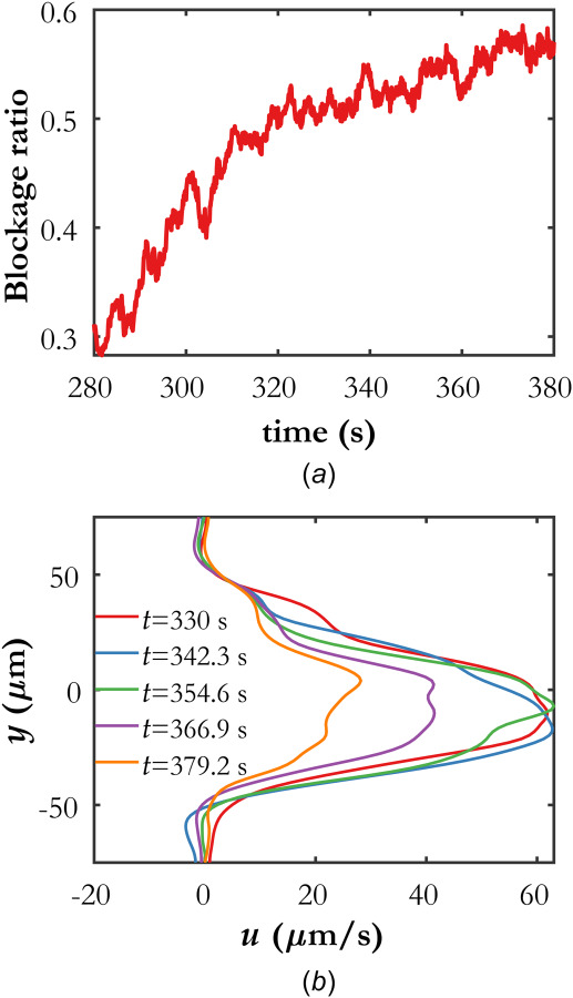
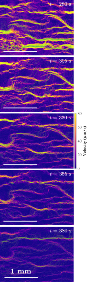
This article describes novel measurements of the velocity of whole blood flow in a microchannel during coagulation. The blood is imaged volumetrically using a simple optical setup involving a white light source and a microscope camera. The images are processed using particle image velocimetry (PIV) and wavelet-based optical flow velocimetry (wOFV), both of which use images of individual blood cells as flow tracers. Measurements of several clinically relevant parameters such as the clotting time, decay rate, and blockage ratio are computed. The high-resolution wOFV results yield highly detailed information regarding thrombus formation and corresponding flow evolution that is the first of its kind.

Fig. 1

Schematic view of the experimental setup. A pressure control unit was utilized to inject the blood sample into the microfluidic channel at a constant pressure of 20 mBar. The microfluidic channel was placed on an inverted microscope, and the blood flow was recorded under 4X magnification using a high-resolution microscope camera.

Fig. 2

Example blood flow images from the 100 mM CaCl₂ case at $t=230-380$ s at intervals of 50 s, showing the development of coagulation. Flow is from left to right. The flow has coagulated in the dark regions of the bottom three images. The images have been preprocessed using the steps described in the text. The horizontal line in the lower left of the image at t = 330 s indicates the scale (1 mm).

Fig. 3

Mean horizontal velocity for each case determined by PIV. The clotting time is observed to be 220 s.

Fig. 4

Instantaneous snapshots of the velocity field at t = 330 s for (a) PIV and (b) wOFV. The velocity field is colored according to velocity magnitude, and the spatial scale is shown in the lower left of each subfigure.

Fig. 5

Instantaneous snapshots of the velocity field at t = 330 s for wOFV showing (a) velocity vectors and (b) streamlines, each shown in green. The velocity field is colored according to velocity magnitude. Velocity vectors are subsampled by a factor of 30 in both dimensions and scaled by a factor of 20 to aid in visualization. The transparency for each streamline is set according to the mean residence time along that streamline, with more transparency indicating a longer residence time (lower average velocity). The vertical white line in (b) is referenced in Fig. 7. The horizontal white lines indicate the spatial scale. A zoomed-in image of the region marked by a red rectangle in (b) shows the streamlines in finer detail.

Fig. 6

Histogram of normalized residence times for the streamlines shown in Fig. 5(b)

Fig. 7

(a) Temporal evolution of the computed blockage ratio, quantified by the number of streamlines that traverse a majority of the domain to the total number of seeded streamline starting locations. (b) Temporal evolution of the horizontal component of velocity along the flow channel marked with a vertical white line in Fig. 5(b). The origin on the y-axis is arbitrary.

Fig. 8

Evolution of the velocity field determined using wOFV as a function of time. Coloration indicates velocity magnitude, and the streamlines are colored according to mean residence time. Horizontal white lines indicate the spatial scale.