The molecular basis for sarcomere organization in vertebrate skeletal muscle

Abstract

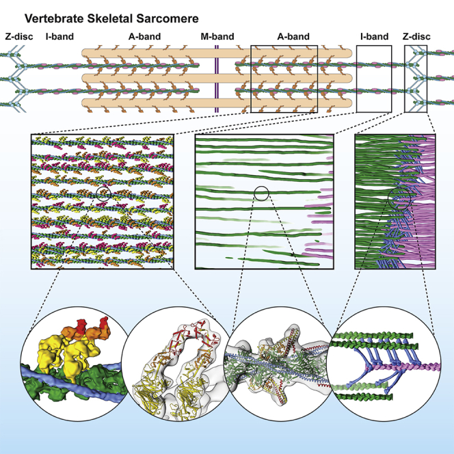
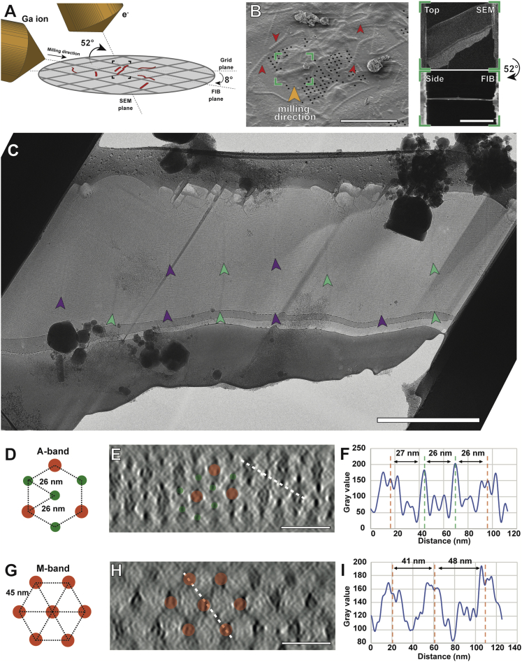
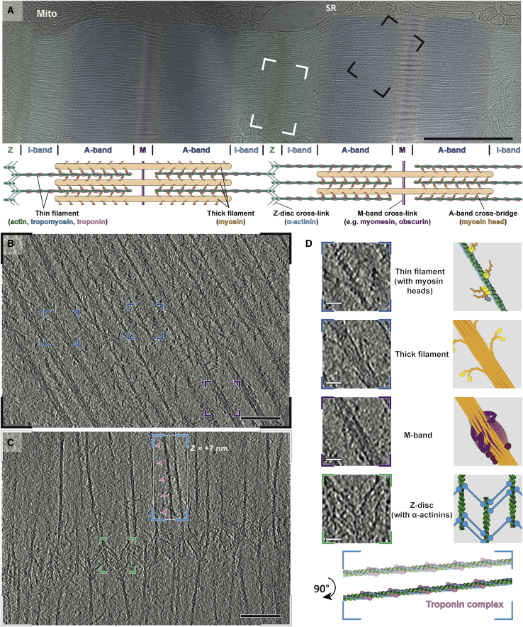
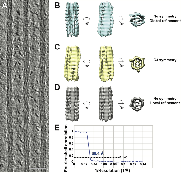
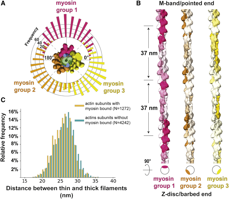
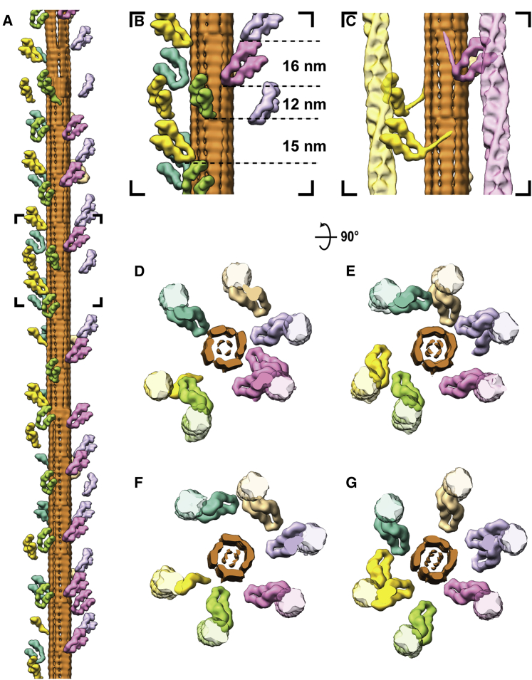
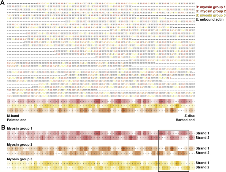
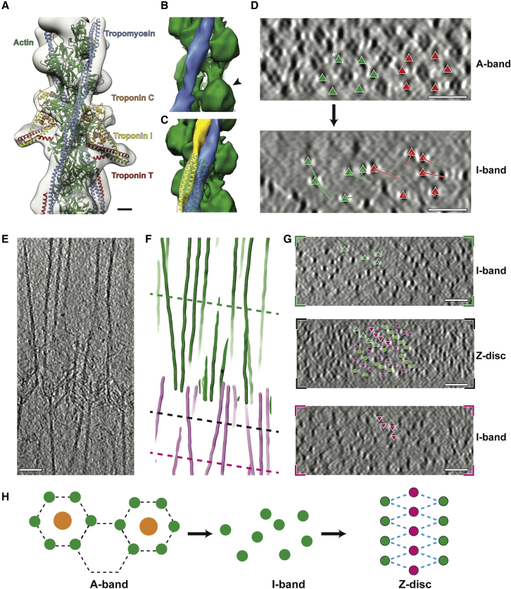
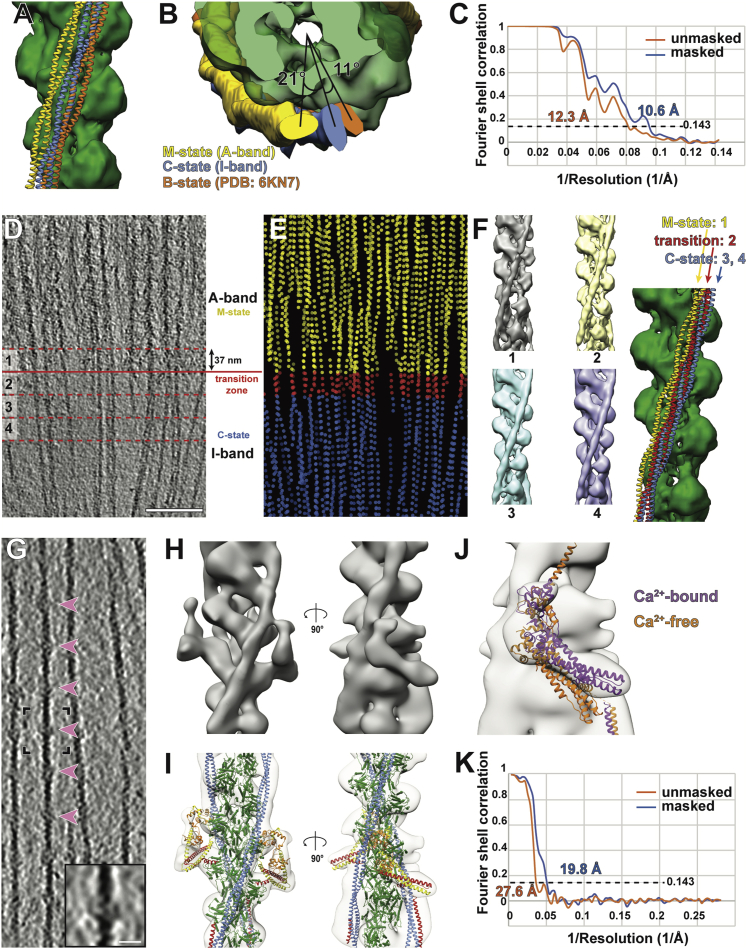
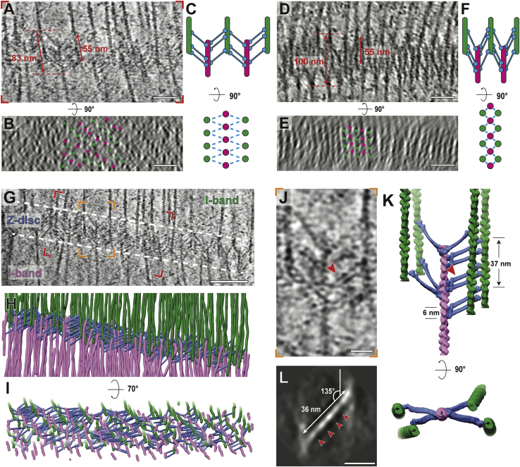
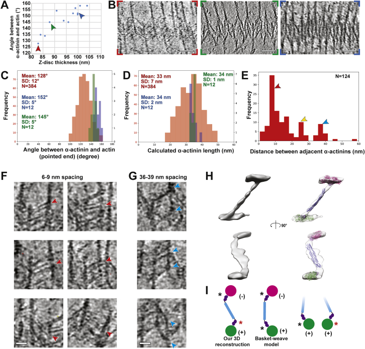
Sarcomeres are force-generating and load-bearing devices of muscles. A precise molecular picture of how sarcomeres are built underpins understanding their role in health and disease. Here, we determine the molecular architecture of native vertebrate skeletal sarcomeres by electron cryo-tomography. Our reconstruction reveals molecular details of the three-dimensional organization and interaction of actin and myosin in the A-band, I-band, and Z-disc and demonstrates that α-actinin cross-links antiparallel actin filaments by forming doublets with 6-nm spacing. Structures of myosin, tropomyosin, and actin at ~10 Å further reveal two conformations of the "double-head" myosin, where the flexible orientation of the lever arm and light chains enable myosin not only to interact with the same actin filament, but also to split between two actin filaments. Our results provide unexpected insights into the fundamental organization of vertebrate skeletal muscle and serve as a strong foundation for future investigations of muscle diseases.

Keywords: Z-disc; actin; electron tomography; muscle; myosin; sarcomere; structure; tropomyosin.

Graphical abstract

Figure S1

Cryo-FIB-ET of isolated mouse myofibrils reveals sarcomere ultrastructure and hexagonal arrangement of filaments in the cross-section view, related to Figure 1 (A) Cartoon showing the arrangement of the SEM and FIB ion source with respect to the grid. Myofibrils are depicted in red. (B) Left: SEM image taken 45° to the plane of a grid on which myofibrils were vitrified, with red arrow heads pointing toward the myofibrils. The orange arrow head indicates the milling direction. Scale bar, 50 μm. Right: Top (taken with electron beam) and side (taken with ion beam) views of the lamella taken after milling in the FIB-SEM. The top view was taken 60° angle to the plane of the grid. The side view was taken 8° to the plane of the grid, which was also the milling angle. Scale bar, 5 μm. (C) Projection image of a lamella after FIB-milling recorded at a TEM at stage 0°. Purple arrow heads indicate M-bands of sarcomeres, while green arrow heads indicate Z-discs. Scale bar, 3 μm. (D and G) Schematic diagrams of the triangular arrangement of thick filaments in the A-band (D) and the hexagonal arrangement of thin filaments in the M-band (G). Thin and thick filaments are represented by green and orange circles, respectively. (E and H) Slices of the cross-section view of tomograms in the A-band (E) and the M-band (H). The tomograms were previously filtered with an equator filter on XY slices in Fourier space to remove signals from cross-bridges. The thicknesses of lamellae were measured in this view. Scale bar, 50 nm. (F and I) Distances between filaments were measured using the line profiles of the white dotted lines in (E) and (H), respectively.

Figure 1

Isolated mouse skeletal myofibrils imaged using electron cryotomography (A) Projection image of mouse skeletal muscle, with Z-disc, I-, M-, and A-bands visible (green, light blue, dark blue, and purple, respectively). A schematic diagram is shown below, highlighting the lateral organization and cross-links in different zones. Mitochondria (Mito) and sarcoplasmic reticulum (SR) can be identified between sarcomeres. Scale bar, 1 μm. (B) Slice through an electron cryo-tomogram spanning A- to M-band. Its representative position on a sarcomere is marked as the black box in (A) (not same sarcomere). In this region, myosin heads bound to the thin filament, myosin tails emanating from the thick filament (dark blue insets) and obscure protein densities at the M-band (purple inset) can be discerned. Scale bar, 100 nm. (C) Slice through an electron cryo-tomogram spanning I-band and Z-disc. Its representative position on a sarcomere is marked as the white box in (A) (not same sarcomere). The tail-feather-like arrangement of α-actinin molecules cross-linking thin filaments in a zig-zag manner is visible (green inset). Thin filaments in the I-band have regularly-spaced nodes corresponding to troponin complexes (pink arrow heads, blue inset). A slice of the same location but 7 nm above from the rest of the slice is shown inset. Scale bar, 100 nm. (D) Larger view of insets described in (A)–(C), with cartoon depictions of densities. Scale bar, 20 nm. See also Figure S1.

Figure S2

Sub-volume averaging of thick filaments, related to Figures 3 and 5 (A) Slice through a tomogram depicting three adjacent thick filaments. Scale bar, 50 nm. (B) Averaged structure from a global refinement. The map suffers from missing wedge artifacts, indicating alignment focused on the missing wedge instead of actual structural features. (C) The distribution of myosin heads when retracted to the thick filaments in the relaxed state has a C3 symmetry. We therefore performed a refinement and reconstruction applying C3 symmetry. However, this did not improve the quality of the map, indicating that the core of vertebrate thick filaments is not C3 symmetric. (D) A local refinement with restricted possible rotation angles reduced alignment errors and thereby missing wedge artifacts. This reconstruction was used as a model for thick filament in Figures 3 and 5. (E) The estimated resolution of the reconstruction in (D) is 30.4 Å using the 0.143 criterion.

Figure S3

Strategies of sub-volume averaging of the in situ actomyosin complex and different “kink” conformations in the lever arm, related to Figure 2 and STAR Methods (A) Workflow of sub-volume averaging leading to the final structures of the in situ actomyosin complex and double-head myosin. Details of the colored steps are shown in (B-G). (B) Examples of selected and discarded 2D class averages. After cleaning by 2D sorting, 21,130 out of 32,421 sub-volumes were selected for subsequent processing. (C) Initial reference and the average after the first 3D refinement with only a spherical mask with a diameter of 340 Å applied. (D) Classes of the actomyosin complex after 3D classification. Prominent myosin double head pairs in each class are indicated by red arrow heads. These pairs were later aligned to each other during merging the classes by modifying the alignment parameters. The classes in the black box were selected and used for subsequent processing. (E) Classes of the myosin double-heads after the 3D classification applied on the sub-volumes re-centered on myosin heads. The two classes in the black boxes showing clear densities for the double-head were selected for the final averaging. (F) Left: final reconstruction of the actomyosin complex generated from the local refinement with a mask around the thin filament and a pair of myosin heads after merging the classes in (D). The map is colored based on local resolution. The purple inset shows the area of the re-centered sub-volumes for double-head analysis in (E) and (G). Right: The estimated resolution of the reconstruction is 10.2 Å using the 0.143 criterion. (G) Left: final average of the complete myosin double-head including RLC. Right: The estimated resolution of the reconstruction is 15.1 Å using the 0.143 criterion. (H) Example details showing secondary structures that are visible in the averaged structure in F. The red arrow heads indicate the D-loop of actin, helix-loop-helix motif and loop 3 of myosin from left to right at the interface between actin and myosin. (I) Alignment of ELCs, together with the ELC-binding region, from different atomic models of myosin heads. Only the RLC-binding helix of the lever arm in each model is shown instead of the complete RLC for clear visualization. Two different groups of conformations are shown. The conformation of the lower head (red) is similar to the relaxed blocked state (orange). The upper head (blue) exhibits a similar conformation to the relaxed free head (purple) and the crystal structure of squid myosin S1 (green). (J) Side-by-side comparison of the complete myosin atomic models in (I) showing the heavy chain and both light chains.

Figure 2

Sub-volume averaging of thin filaments reveals the interaction of a double-head myosin with the thin filament and two conformations of light chain domains within a double-head (A) Surface view of the in situ actomyosin structure, showing actin filament (green), tropomyosin (blue), and myosin double heads, with motor domains (yellow), essential light chains (orange), and regulatory light chains (red). Scale bar, 5 nm. (B) Close-up view of the lower myosin head and homology models based on PDB: 3I5G, 5JLH, and 6KN8. The upper 50 kDa (U50), lower 50 kDa (L50), SH3, and essential light chains (ELC) can be allocated in the map, along with part of the regulatory domain (RLC). Arrow heads indicate the interaction interfaces between actin and myosin at loop 4, helix-loop-helix motif, loop 3 of myosin (top to bottom). Arrow heads in the inset depict interaction interfaces at the cardiomyopathy loop and loop 2 (left to right). (C) Close-up of an actin subunit and structural model fitted into the EM map showing the four subdomains of an actin subunit (SD1–SD4). (D) Surface view of the structure of a complete myosin double-head including RLCs determined from averaging shifted sub-volumes (see Figure S4). Their interface is indicated by a dotted line. (E) Comparison between the lower and upper heads within one double head, showing two different conformations in the lever arm that interacts with RLC and ELC. Lengths of the lever arms were measured between G772 and L844. (F) Alignment of the lower (purple) and upper (blue) heads heavy chain, showing two different kinks between the ELC-binding region and the RLC-binding region. See also Figures S2 and S3.

Figure 3

Organization of the A-band in natively isolated myofibrils shows that myosin heads can adopt two interactions with thin filaments (A) XY-slices through a tomogram at three different Z positions (illustrated by the cartoon below), highlighting the myosin head densities (orange, yellow, and magenta) and the thin filament (green) apparent within the volume. Annotation of densities produces a volume in which filtered actomyosin can be fitted, shown on the right and in (B). The three myosin colors represent the contribution of the myosin head from a respective neighboring thick filament. Scale bars, 20 nm. (B) Fitted model of all thin filaments and myosin heads in a tomogram, with the black inset depicting the filament shown in (A) In the XZ view, reconstructions of corresponding thick filaments are also shown. (C) A typical cross-bridge with a myosin double-head. (D) A rare myosin split-head with two heads from the same myosin molecule binding to two different actin filaments. See also Figures S2 and S4 and Video S1.

Figure S4

Annotation and fitting of split and double heads of myosin between thin and thick filaments from A-band tomograms, related to Figures 3 and 5 (A) Annotated density of a thin filament including the myosin heads (green), with the annotated density for a myosin double-head highlighted in orange. (B) Oblique and zoomed-in view of the double-head density and its associated thick filament segmentation (pink). (C) Same view as in (B) including the fitted thin filament and myosin double-head models from sub-volume averaging. (D) Annotated density of two thin filaments including the myosin heads (green and light blue), highlighting annotated density corresponding split-head in orange. (E) Oblique and zoomed-in view of the split-head density and its associated thick filament segmentation. (F) Same view as in (E) including the fitted thin filament and myosin split-head models. The split-head is composed of two heads in the upper head conformation in order to be fitted into the density.

Figure 4

Myosin binding preference is dependent on actin orientation and distance between thin and thick filaments (A) Angular distribution of myosin heads shown by a circular histogram of the orientation of the actin subunits bound by myosin heads. The colors indicate three different thick filaments where the myosin heads originate. (B) Hotspots of myosin binding from three thick filaments shown on actin filaments. Actin filaments are colored with the footprint of the myosin heads according to multiple sequence alignment of the myosin binding profile sequences determined from the annotated volume and the fitted model in Figure 3B. See also Figure S5. The preferred side on a thin filament for binding of a certain myosin group is shown in the schematic diagram below. (C) Histograms of distances between thin and thick filaments at actin subunits with (orange) or without (green) a myosin head bound. Mean distances are 25.9 nm (SD 2.7 nm) and 26.3 nm (SD 2.7 nm), respectively. No skewness was measured in either population, meaning both distributions can be considered Gaussian.

Figure 5

Arrangement of myosin heads around a thick filament (A) Model of a thick filament with surrounding thin filament-bound myosin heads obtained from fitting into the annotated tomogram. The six different colors represent myosin heads bound to the six adjacent thin filaments. (B) Close-up view of the black inset in (A) showing varying spacings between the tips of adjacent myosin heads. (C) Different conformations of S2 fragments taken from clearly discernible annotations. (D–G) Top view of four segments of the thick filament in (A) together with the thin filaments it binds, highlighting heterogeneity of myosin head organization. Each image depicts a segment with a depth of ~40 nm. See also Figures S2 and S4 and Video S1.

Figure S5

Overall myosin binding profile generated from multiple sequence alignment of myosin binding profiles of 30 thin filaments, related to Figure 4 and STAR Methods (A) The fitted myosin head model in Figure 3B was converted to myosin binding profile sequences on thin filaments, with “R,” “G,” “B” representing actin subunits bound by three groups of myosin heads originating from three neighboring thick filaments and “E” representing myosin-free actin subunits. These sequences were aligned using multiple sequence alignment with a customized weight matrix. Only the sequence of one actin strand for each thin filament was used for alignment. The sum of occurrence of each myosin group at each actin subunit position is shown at the bottom and colored accordingly. Darker color indicates higher occurrence. (B) The colored overall myosin binding profile on both actin strands for each myosin group. Sequences of strand 2 were combined using the alignment of strand 1 shown in (A). The overall myosin binding profiles depict hotspots for myosin binding on a thin filament and the region highlighted in the black box is used to color the models shown in Figure 4B.

Figure 6

Structure and organization of thin filaments in the I-band (A) Sub-volume average of the thin filament in the I-band fitted with a homology model of the complete thin filament including troponin. Homology model is based on PDB: 6KN8. (B) 3D reconstruction of the thin filament in the I-band excluding troponin. The actin filament is depicted in green and tropomyosin in blue. At this resolution, the four subdomains of actin form a clear “U” shape (marked by the arrow head) and indicates actin barbed end faces toward the Z-disc. (C) Tropomyosin along thin filaments takes the C-state in the I-band (blue) and the M-state in the A-band (yellow). (D) XZ views of sarcomeres at the A-band and I-band highlighting the disappearance of the hexagonal pattern of thin filaments. Two hexagonal units of thin filaments and their corresponding positions in the I-band are indicated by green and orange triangles. Displacement of the filaments from A-band to I-band are shown as arrows. Asterisk denotes a filament that moved out of the field of view during the A–I transition. (E) Slice through a tomogram depicting the Z-disc and two I-bands from two adjacent sarcomeres. (F) 3D model of thin filaments showing the same region as in (E). (G) Cross-section views of the positions indicated by dotted lines in (F), showing the pattern of thin filaments during the I-Z-I transition. Filaments are traced in green triangles from the I-band to Z-disc of the top sarcomere and in magenta triangles from the Z-disc to the I-band of the bottom sarcomere. In the Z-disc image, antiparallel filaments in the center are labeled with green and magenta dots. (H) A schematic diagram shows the hexagonal pattern in the A-band, the irregular pattern in the I-band and the rhomboid pattern in the Z-disc. Scale bars, 2 nm (A), 50 nm (D–G). See also Figure S6.

Figure S6

Sub-volume averaging of the thin filaments in the I-band, related to Figure 6 (A and B) Comparison of tropomyosin positions in different regions of the sarcomere. Side (A) and top (B) views of a thin filament with tropomyosin in the A-band (yellow) and I-band (blue). Tropomyosin is in the M state in the A-band and resides in the C-state in the I-band. The two states differ by an azimuthal rotation of ~21°. The B-state tropomyosin from a model of Ca²⁺-free thin filament (PDB: 6KN7) (orange) is also shown for comparison. (C) The estimated resolution of the reconstruction of a thin filament excluding troponin in the I-band is 10.6 Å using the 0.143 criterion. (D) Slice from a tomogram showing both A-band and I-band. The solid red line represents the border between the A-band and I-band. 37-nm sections separated by the red dotted lines were selected for separate sub-volume averaging. (E) 3D view of particles of the thin filaments in the same region as (D), colored based on the state of their tropomyosin position. All A-band particles exhibit the M-state tropomyosin position (yellow). Most I-band particles exhibit the C-state tropomyosin (blue). The particles in the closest 37-nm section in the I-band to the A-band (section 2 in (D)) exhibit an intermediate position of tropomyosin, and hence define a transition zone. (F) Averaged structures corresponding to sections 1-4 as indicated in (D). The structures were aligned to a non-decorated F-actin structure. Tropomyosin models fitted into the structures are shown on the right. Section 1 has the same tropomyosin position as the M-state structure. Section 3 and 4 has the same tropomyosin position as the C-state structure. Section 2 has an intermediate tropomyosin position between the M- and C-state, implying that this is the section where the transition occurs. (G) Slice of a tomogram depicting thin filaments in the I-band. Bulges along the filaments appear with a periodicity of ~37 nm (highlighted by pink arrow heads), corresponding to troponin complexes. An enlarged version of a pair of troponin complexes in the black inset is shown at the bottom-right corner, depicting clear extra densities. Scale bar, 10 nm. (H) 3D reconstruction of a thin filament decorated by a pair of troponin complexes obtained from sub-volume averaging. (I) A homology model based on the structure of the Ca²⁺-bound cardiac muscle thin filament (PDB: 6KN8) was fitted into the map. Actin, tropomyosin, troponin I, troponin T and troponin C are shown in green, blue, yellow, red, and orange, respectively. (J) The structure of troponin in the Ca²⁺-bound state (PDB: 6KN8) fits much better into the map than the structure of troponin in the Ca²⁺-free state (PDB: 6KN7). Together with the C-state position of tropomyosin (A and B), this indicates that the I-band thin filament is in the Ca²⁺-bound state. (K) The estimated resolution of the reconstruction of the thin filament including troponin in the I-band is 19.8 Å using the 0.143 criterion.

Figure 7

Different types of Z-discs from fast mouse psoas myofibril and α-actinin organization in the thinner form (A–C) XY slice view (A), equator-filtered cross-section view (B), and a schematic diagram showing the pattern (C) of a Z-disc in the thinner form within a tomogram. The thickness of the Z-disc was measured between where α-actinins bind to the antiparallel thin filaments. The length of a single thin filament within the Z-disc was also measured. The organization of the filaments in this Z-disc is rhomboidal, likely resulting from a tilted orientation of the Z-disc on the grid and a slight stretching of the myofibril. We used this Z-disc for our analysis because most of the α-actinin densities could be unambiguously assigned. Scale bar, 50 nm. (D–F) XY slice view (D), cross-section view (E), and a schematic diagram of a tomogram showing a Z-disc in the thick form with a square pattern (F). This is the predicted organization of a Z-disc from skeletal muscle. However, it is difficult to assign individual α-actinin densities in these tomograms hampering a non-biased annotation. Scale bar, 50 nm. (G) Slice through the same tomogram as (A) depicting the thin-form Z-disc and two I-bands. Scale bar, 100 nm. (H) Cryo-ET based 3D model of the Z-disc showing antiparallel thin filaments from two adjacent sarcomeres (green and magenta) and the α-actinins (blue) cross-linking the filaments. (I) Tilted view of the model shown in (H). (J) Slice of an example unit in the Z-disc depicting one thin filament with its neighboring antiparallel thin filaments and the α-actinins connecting them. A doublet of α-actinins is highlighted by a red arrow head. Scale bar, 20 nm. (K) Cryo-ET-based 3D model of the same region in (J). Actin filament model is derived from the thin filament reconstruction in Figure 6A, excluding tropomyosin. The α-actinin model is derived from the crystal structure of an α-actinin dimer (PDB: 4D1E). (L) Projection image (7-nm thickness) of the 3D reconstruction of α-actinin obtained from averaging the sub-volumes as picked in (H) and (I), depicting four domains (marked by red arrow heads) which correspond to the four spectrin-like repeats (SRs) in the rod region. Scale bar, 20 nm. See also Figure S7 and Video S2.

Figure S7

α-Actinin structure and organization in the Z-disc, related to Figure 7 (A) Plot relating the thickness of Z-discs and the angle between α-actinins and the pointed end of actin filament from different tomograms. The positive correlation implies a parallel hinge mechanism of the Z-disc. (B) Slices through tomograms depicting a thin Z-disc (left, red arrow in (A)), a thick Z-disc (right, blue arrow in (A)) and a Z-disc of intermediate thickness (middle, green arrow in (A)). Scale bar, 50 nm. (C) Distribution of the calculated angles between annotated α-actinins and actin filaments in direction to the pointed end in the thin (red), thick (blue) and intermediate-thickness (green) Z-discs. The y axis for both the thick and intermediate Z-disc is shown on the right in black. There are more data points for the thin Z-disc as it was completely annotated, while a few examples of α-actinin were selected for the intermediate and thick Z-discs. (D) Distribution of the length of annotated α-actinins in the thin (red), thick (blue) and intermediate-thickness (green) Z-discs. The distance along α-actinin between the centers of the connecting actin filaments was measured and the length of α-actinin was calculated by subtracting the diameter of an actin filament (6 nm). The relatively large standard deviation in the thin form Z-disc is likely caused by α-actinins binding to actin filaments at different azimuthal orientations and the error in the precise determination of the central axis of actin filaments. (E) Distribution of the calculated spacing between adjacent α-actinins in the thin Z-disc. The red, yellow, and blue arrow heads highlight peaks at 6-9 nm, 24-27 nm and 36-39 nm, respectively. The 24-27 nm peak appears as a result of the two other types of spacing (36 - 2x6). (F and G) Example images showing α-actinins with the 6-9 nm spacing (D) and the 36-39 nm spacing (E). Arrow heads highlight the positions and orientations of α-actinins. Scale bar, 20 nm. (H) 3D reconstruction of α-actinin obtained from sub-volume averaging. Although there is a strong missing wedge effect resulting in an elongation of the reconstruction in one direction, we were able to manually fit atomic models derived from the crystal structure of α-actinin (PDB: 4D1E) and the cryo-EM structure of actin filaments bound by the first calponin homology domain of the actin binding domain (PDB: 6D8C) into the density. Actin filaments are shown in magenta and green; the actin binding domain and the rod region are depicted in purple and blue, respectively. The flexible neck regions and the C-terminal calmodulin-like domains are not shown. (I) Left: Schematic diagram showing the difference between averaged α-actinin structure and the conventional basket-weave model. Right: The two different interactions (marked by the red and black asterisks) between the end of α-actinin and actin filaments (magenta and green) are demonstrated on the right, formed by the flexible neck region between the rod (blue) and actin binding domain (purple).

References

1. Al-Khayat H.A., Squire J.M. Refined structure of bony fish muscle myosin filaments from low-angle X-ray diffraction data. J. Struct. Biol. 2006;155:218–229. - PubMed
1. AL-Khayat H.A., Hudson L., Reedy M.K., Irving T.C., Squire J.M. Myosin head configuration in relaxed insect flight muscle: x-ray modeled resting cross-bridges in a pre-powerstroke state are poised for actin binding. Biophys. J. 2003;85:1063–1079. - PMC - PubMed
1. Al-Khayat H.A., Kensler R.W., Squire J.M., Marston S.B., Morris E.P. Atomic model of the human cardiac muscle myosin filament. Proc. Natl. Acad. Sci. USA. 2013;110:318–323. - PMC - PubMed
1. Alamo L., Wriggers W., Pinto A., Bártoli F., Salazar L., Zhao F.Q., Craig R., Padrón R. Three-dimensional reconstruction of tarantula myosin filaments suggests how phosphorylation may regulate myosin activity. J. Mol. Biol. 2008;384:780–797. - PMC - PubMed
1. Baumann B.A.J., Taylor D.W., Huang Z., Tama F., Fagnant P.M., Trybus K.M., Taylor K.A. Phosphorylated smooth muscle heavy meromyosin shows an open conformation linked to activation. J. Mol. Biol. 2012;415:274–287. - PMC - PubMed
Publication types