Artificial intelligence in OCT angiography

Abstract

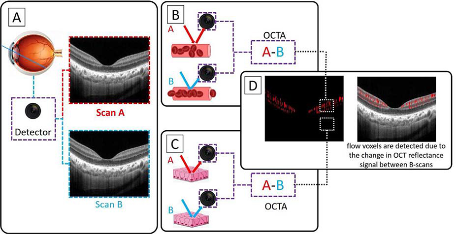
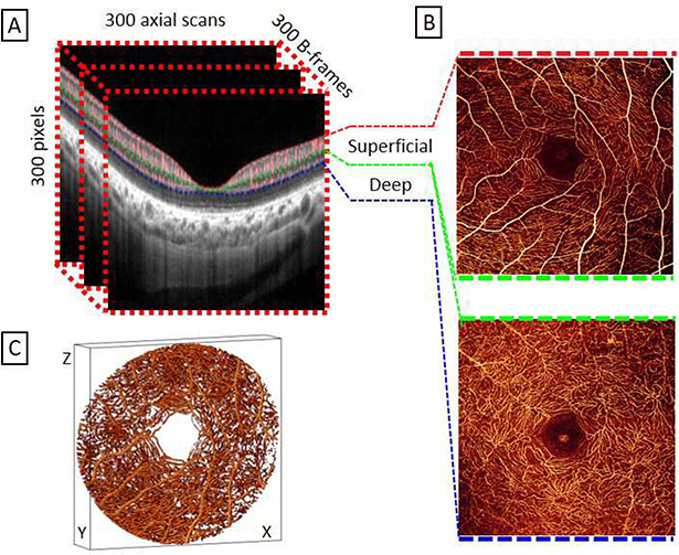
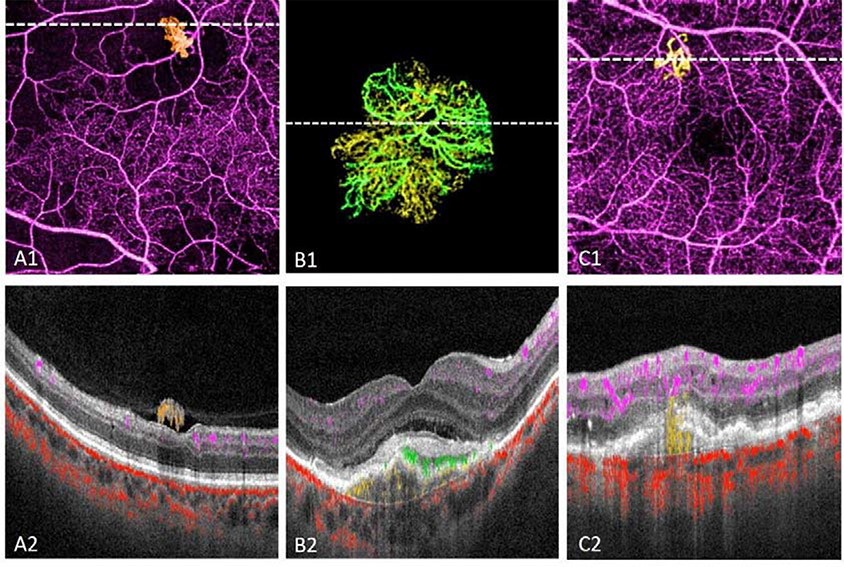
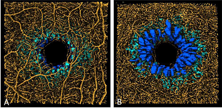
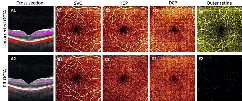
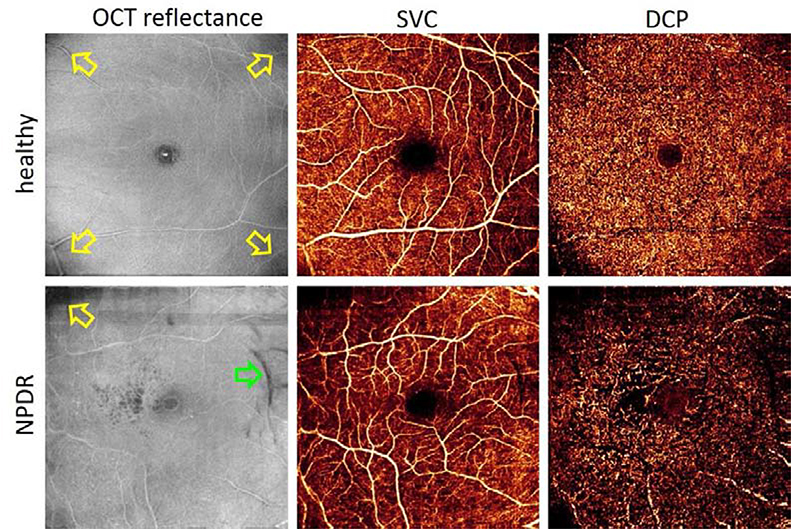
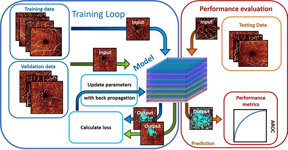
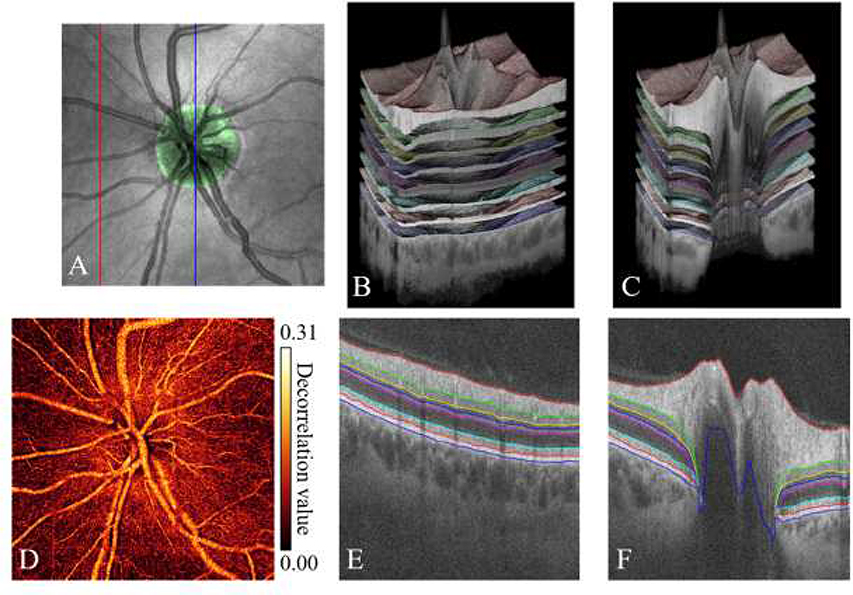
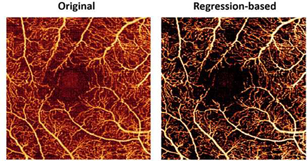
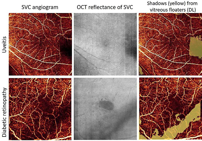
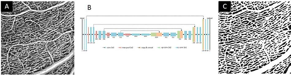
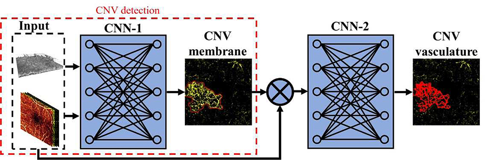
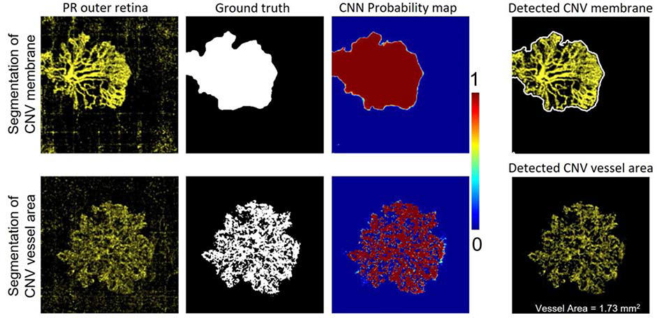
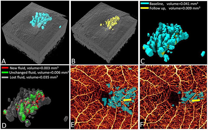
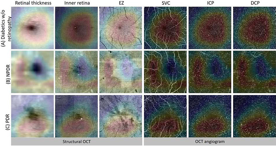
Optical coherence tomographic angiography (OCTA) is a non-invasive imaging modality that provides three-dimensional, information-rich vascular images. With numerous studies demonstrating unique capabilities in biomarker quantification, diagnosis, and monitoring, OCTA technology has seen rapid adoption in research and clinical settings. The value of OCTA imaging is significantly enhanced by image analysis tools that provide rapid and accurate quantification of vascular features and pathology. Today, the most powerful image analysis methods are based on artificial intelligence (AI). While AI encompasses a large variety of techniques, machine-learning-based, and especially deep-learning-based, image analysis provides accurate measurements in a variety of contexts, including different diseases and regions of the eye. Here, we discuss the principles of both OCTA and AI that make their combination capable of answering new questions. We also review contemporary applications of AI in OCTA, which include accurate detection of pathologies such as choroidal neovascularization, precise quantification of retinal perfusion, and reliable disease diagnosis.

Keywords: Artificial intelligence; Deep learning; Image analysis; OCT Angiography.

Figure 1.

OCTA signal generation schematic. (Panel A) An OCTA imaging procedure captures two cross-sectional structural OCT scans, scan A and scan B. (B) When the OCT sample beam encounters a blood vessel, scan A and scan B produce different signals, since the sample beam interacts with a dynamic structure. (C) On the other hand, when the sample beam encounters static tissue, the signals from scan A and scan B are identical. (D) The OCTA signal can be generated by the absolute difference between scans A and B. For beams encountering static tissue this difference is small, while for flow tissue it is large. Since it is constructed from the OCT reflectance signal, OCTA images are automatically co-registered with structural OCT images, so that the location of retinal vasculature can be readily compared to other anatomic features.

Figure 2.

OCTA data representations. (A) Cross-sectional images can be generated from individual B-frames, or by projecting several B-frames to form a composite image. In the example images here, three anatomic slab boundaries are colored red, green, and blue. (B) The flow signal can be projected between these boundaries to create en face representations, which are akin to color fundus photography and dye-injection angiography images. (C) Since OCTA is a three-dimensional imaging modality, volume renderings can also be used.

Figure 3.

En face and cross-sectional OCTA representations highlighting retinal neovascularization (RNV), choroidal neovascularization (CNV), and retinal angiomatous proliferation (RAP). In each image, the flow signal is color coded according to its position (orange: vitreous; violet: inner retina; yellow: outer retina, red: choroid). (A) The RNV lesion can be clearly located in the en face and cross-sectional images due to its location in the vitreous. (B) Here, the outer retinal vessels are additionally colored according to location relative to the retinal pigment epithelium (green: above, yellow: below). This enables easy identification of type 1 (yellow) and type 2 (green) CNV, and can help identify mixed lesions such as the example here. (C) A cross-sectional view clearly shows the RAP vessels extending between the choroid and outer retina. In all of the examples shown, both the en face and cross-sectional images can help to identify and characterize the pathology.

Figure 4.

Volume renderings of an eye with a macular hole. (A) View looking down from the superficial vascular complex, and (B) looking up from the deep capillary plexus. Blue indicates intra-retinal cystoid spaces, with light blue indicating a location in the inner nuclear layer and dark blue between the outer plexiform layer and Henle’s fiber layer. Volumetric representations can avoid misleading images in which extended fluid volumes may appear small due to their projected area in cross-sectional or en face images.

Figure 5.

Projection artifacts and their removal from 6×6-mm OCTA images. (Top row) Uncorrected OCTA data includes projection artifacts in both cross-sectional and en face images. (A1) In cross-section, projection artifacts manifest as tails extending below vessels. In this image, the flow signal is overlaid on the structural image (gray scale), and colored according to anatomic depth (violet: inner retina, yellow: outer retina, red: choroid). In en face images, the flow signal from the superficial vascular complex (SVC; B1) is duplicated in the intermediate capillary plexus (ICP; C1), deep capillary plexus (DCP; D1) and the outer retina (E1), which is avascular in healthy eyes. (Bottom row) Projection-resolved OCTA (PR-OCTA) removes projection artifacts in both cross-sectional and en face images.

Figure 6.

Shadowing artifacts. En face images of a healthy volunteer (top row) shows shadows caused by vignetting (yellow arrows) in the OCT reflectance channel (left column), superficial vascular complex (SVC), and deep capillary plexus (DCP). The shadowing artifacts are more prominent in the deeper layers. Vignetting as well as a shadow due to a vitreous floater (green arrow) are apparent in an eye with non-proliferative diabetic retinopathy (NPDR; bottom row).

Figure 7.

Microsaccadic artifacts and their removal. Scanning along a priority axis will produce Fast X and Fast Y scans, in which microsaccades manifest as bright lines in the scanning direction. These artifacts can be corrected by registering and merging the images, as shown in the motion correction technology (MCT) image. However, note some residual artifacts still present in the MCT image.

Figure 8.

Training and evaluation in machine learning (schematic). The goal of a learning algorithm (portrayed as a convolutional neural network labeled “model”, above) is to achieve adequate performance on previously unseen data in a specific task by learning from a training data set. Here, an example of training a network to segment non-perfusion area in an OCTA en face image is shown. During training (training loop panel above) the training data is input to the model (blue arrows). The model’s output on the training data is compared to a benchmark or ground truth, with its performance evaluated by means of a loss function. By updating parameter values to minimize the loss, the network can learn features in the data and improve its performance on the training data. Most networks can achieve reliable results on training data, but the real question is if the network can generalize to perform the same task on unseen data, like images of a new patient. To assess generalizability a validation data set is often also included in the training data (green arrows). The validation set is characterized during the training process the same as the training data, but the results are not used in parameter updates. In this way generalizability can be gauged during training, since the model does not learn the validation set. To fully assess generalizability, a unique testing data set is used (performance evaluation panel; orange arrows). Here, the network’s performance is evaluated with metrics like the area under receiver operating characteristic curve (AROC).

Figure 9.

Simple U-net-like convolutional neural network (CNN). U-nets form the basis of many state-of-the-art image segmentation algorithms. Following the green arrows in the network diagram above indicates where this network architecture got its name. U-nets are often employed in medical imaging to perform semantic segmentation. In the encoder arm, the input image is downsampled with max pooling layers in order to help learn features. In the decoder arm, the learned feature maps are upsampled to produce a segmented image the same size as the input. In U-nets skip connections (purple arrows) concatenate feature maps in the encoder arm’s outputs to outputs in the decoder arm. These skip connections help the network to maintain resolution in the segmented output. Blue and red numbers next to the network layers indicate the size of the input data at each layer and the number of output feature channels, respectively.

Figure 10.

Example resnet-like module. Resnets form the basis of many state-of-the-art image classification networks. In Resnets, skip connections (purple arrows) link the outputs of shallower convolution layers (blue layer) with deeper through addition. Multiple modules such as the one pictured can be chained together to create very deep networks, before the output is determined by a decision making layer (red layer).

Figure 11.

OCTA signal generation from a single B-frame using deep learning. (A) A macular OCTA image from a Zeiss Angioplex instrument. (B) A flow map of the same eye generated by deep learning (DL). The ability to generate OCTA-like data from single B-frames would improve on image acquisition times. Reprinted with permission from (Lee et al., 2019).

Figure 12.

En face OCTA image reconstruction using a convolutional neural network (CNN). (Top row): Original 6×6-mm OCTA en face images of a patient with severe proliferative diabetic retinopathy (PDR), mild non-proliferative diabetic retinopathy (NPDR), a diabetic without retinopathy, and a healthy volunteer. (Bottom row): Equivalent images after reconstruction using a CNN. The CNN used in this work was trained to reconstruct low definition 6×6-mm OCTA images by optimizing a structural similarity loss function which minimized the difference between the original 6×6-mm image and a registered high definition 3×3-mm en face image of the same eye. Arrows in column 1 indicate pathology (microaneurysms: blue; venous beading: green) that was preserved in the reconstructed angiogram.

Figure 13.

Peripapillary Retinal slab segmentation using a convolutional neural network. (A) En face average projection, with the segmented optic disc region overlaid in green. (B) Anatomical map of the entire volumetric OCT based on the segmented peripapillary retinal layers. (C) Cutaway from (B) at the blue line location in (A), clearly showing the anatomic structure inside the disc. (D) En face superficial vascular complex angiogram based on these segmented boundaries. (E) B-frame corresponding to the red line in (A) with segmented peripapillary retinal boundaries. (F) Corresponding image for the blue line in (A). The slab boundaries are, from top to bottom, the vitreous/inner limiting membrane (red), nerve fiber layer/ganglion cell layer (green), inner plexiform layer/inner nuclear layer (yellow), inner nuclear layer/outer plexiform layer (blue), outer plexiform layer/outer nuclear layer (magenta), outer nuclear layer/ellipsoid zone (cyan), ellipsoid zone/retinal pigment epithelium (red) and retinal pigment epithelium/bruchs membrane (blue). Reprinted with permission from (Zang et al., 2019).

Figure 14.

Regression-based bulk motion subtraction. In the original image, the large background is due to the presence of bulk motion. In the regression-based corrected image, the bulk motion has been removed, leading to a larger contrast between the vasculature and surrounding tissue.

Figure 15.

Shadowing artifact detection using deep learning. Shown are an eye with uveitis (top row) and diabetic retinopathy (bottom row). The approach used in this work detected shadowing artifacts using a random forest model taking en face OCTA and OCT reflectance images of the superficial vascular complex (SVC) as input (Camino et al., 2019). The combination of both the structural OCT and OCTA data is a powerful means for intelligent algorithms to identify shadows, since they can learn that shadows coincide in both channels.

Figure 16.

Vessel segmentation using a deep learning. Here, the input (A) consists of a quadrant cropped from a 6×6-mm OCTA en face image. (B) The network architecture used in this study was U-net-like, with skip connections between an encoder and decoder arm. (C) The network outputs a binary vessel map. The segmentation produced by this network improved perfusion quantification in diabetic retinopathy. Adapted with permission from (Heisler et al., 2019)

Figure 17.

Artery and vein classification using deep learning. (A) A raw 4.5×4.5-mm, 400×400-pixel OCTA en face image of the optic nerve head. This image serves as the input to an image reconstruction deep learning (DL) network. (C) The DL reconstructed image is used as the input to another DL network, this one trained to identify arteries and veins form a manually delineated ground truth.

Figure 18

Network architecture (Guo et al., 2019) for a non-perfusion area (NPA) segmentation algorithm. Inputs to the model include a retinal thickness map (A), as well as structural OCT (B) and OCTA (C) en face images of the superficial vascular complex. (A) and (B) are fed into a convolutional neural network (CNN) that learns to extract features relevant for shadow detection, while (C) is fed to a separate network that learns features associated with NPA. The output from each of these networks is then used as input to a series of three parallel CNNs that vote to determine whether a region is NPA (blue), shadow (yellow), or vascular.

Figure 19.

Non-perfusion area (NPA) detection using a convolutional neural network (CNN) (Guo et al., 2019). Shown are an eye with diabetes but not retinopathy, and eye with moderate non-proliferative diabetic retinopathy, and an eye with severe diabetic retinopathy. Column 1 shows unmodified superficial vascular complex (SVC) angiograms, while column 2 shows an expert generated ground truth (green), and column 3 shows the network output. The CNN is capable of distinguishing NPA (blue) from shadowing artifacts (yellow), despite their similar appearance.

Figure 20.

Non-perfusion area detection using deep learning (Wang et al., 2020b). (Top row) En face OCTA images of and eye with severe non-proliferative diabetic retinopathy shows large non-perfusion areas in the deep (DCP) and intermediate (ICP) capillary plexuses, and especially in the superficial vascular complex (SVC). (Bottom row): A neural network outputs the probability that a pixel is part of a non-perfusion area (teal).

Figure 21.

Choroidal neovascularization detection and segmentation network architecture. In order to help distinguish CNV from projection artifacts, the network takes a raw inner retinal angiogram and raw, slab-subtracted, and projection-resolved (PR) outer retinal angiograms, and volumetric structural data from the outer retina as input. A CNN trained to segment the CNV lesion area diagnoses CNV based on the measured lesion size. If a lesion is detected, a second CNN will segment the CNV vessels. Reprinted with permission from (Wang et al., 2020a).

Figure 22.

CNV detection and vessel segmentation using deep learning according to Wang et al. (Wang et al., 2020a). Shown are two example images of CNV. In the top row, the CNV detection network was trained on a ground truth consisting of a segmented membrane area. It outputs an area similar to the ground truth with high probability. The network output consists of a segmented lesion area and a diagnosis of CNV if the detected membrane area exceeds a threshold value. The vessel segmentation network uses the membrane segmentation as input, and was trained on manually traced CNV vessels. It also outputs shapes similar to the ground truth with high probability. The vessel segmentation can be used to determine quantities such as the total vessel area.

Figure 23.

AI-aided retinal fluid detection using structural OCT and OCTA data (Guo et al., 2020). This model segments retinal fluid from densely sampled volumes. (A-B) Automatically segmented retinal fluid at baseline (A; teal) and after treatment followup (B; yellow). (C) Overlaid fluid volumes. (D) The difference in volume at follow up shows that fluid volume has decreased. (E-F) En face OCTA images with fluid area overlaid. The combination of features shows vascular remodeling to avoid fluid volumes (yellow arrow).

Figure 24.

Class activation maps (CAMs) for diabetic retinopathy (DR) classification. Shown are eyes correctly predicted by a convolutional neural network (CNN) as being diabetic without retinopathy (top row), having non-proliferative DR (middle row), and having proliferative DR (bottom row). This network, DcardNet, takes three structural OCT images (the retinal thickness map, and en face images of the ellipsoid zone and retina) and three OCTA images (the superficial vascular complex and intermediate and deep capillary plexuses) as input. The CAMs overlaid atop these inputs show which regions of the image the network considered important (red) or not (blue) for decision making; regions which the network paid attention to can coincide with known features. Reprinted with permission from (Zang et al., 2020).

References

1. Agemy SA, Scripsema NK, Shah CM, Chui T, Garcia PM, Lee JG, Gentile RC, Hsiao YS, Zhou Q, Ko T, Rosen RB, 2015. Retinal vascular perfusion density mapping using optical coherence tomography angiography in normals and diabetic retinopathy patients. Retina 35, 2353–2363. 10.1097/IAE.0000000000000862 - DOI - PubMed
1. Ahlers C, Simader C, Geitzenauer W, Stock G, Stetson P, Dastmalchi S, Schmidt-Erfurth U, 2008. Automatic segmentation in three-dimensional analysis of fibrovascular pigmentepithelial detachment using high-definition optical coherence tomography. Br. J. Ophthalmol. 92, 197–203. 10.1136/bjo.2007.120956 - DOI - PubMed
1. Al-sheikh M, Tepelus TC, Nazikyan T, Sadda SRVR, 2017. Repeatability of automated vessel density measurements using optical coherence tomography angiography. Br. J. Ophthalmol. 101, 449–452. 10.1136/bjophthalmol-2016-308764 - DOI - PubMed
1. Alam Le, Lim Chan, Yao, 2019. Supervised Machine Learning Based Multi-Task Artificial Intelligence Classification of Retinopathies. J. Clin. Med. 8, 872. 10.3390/jcm8060872 - DOI - PMC - PubMed
1. Alam M, Le D, Son T, Lim JI, Yao X, 2020a. AV-Net: deep learning for fully automated artery-vein classification in optical coherence tomography angiography. Biomed. Opt. Express 11, 5249. 10.1364/boe.399514 - DOI - PMC - PubMed
Publication types