The role of kinematic properties in multiple object tracking

Abstract

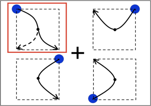
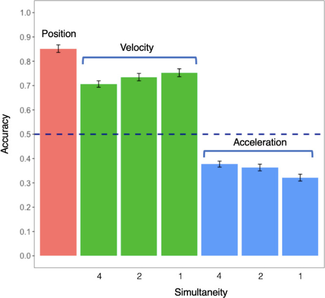
People commonly track objects moving in complex natural displays and their performance in the multiple object tracking paradigm has been used to study such visual attention for more than three decades. Given the theoretical and practical importance of object tracking, it is critical to understand how people solve the correspondence problem to track objects; however, it remains unclear what information people use to achieve this feat. In particular, although people can track multiple moving objects based on their positions, there is ambiguity about whether people can track objects via higher order kinematic information, such as velocity. We designed a paradigm in which position was rendered uninformative to directly examine whether people could use higher order kinematic information to track multiple objects. We find that people can track via velocity, but not acceleration, even though observers can reliably detect the acceleration cue that they cannot use for tracking. Furthermore, we show a capacity constraint on using higher order kinematic information-people perform worse when required to use velocity to resolve correspondence for multiple object pairs simultaneously. Together, our results suggest that, although people can use higher order kinematic information for object tracking, precise higher order kinematic information is not freely available from the early visual system.

Figure 1.

The general set-up of the Experiment 1. (a) Eight objects were displayed as four pairs and each pair had one target and one distractor. (b) Within each quadrant, the target and the distractor were randomly initialized at one of the four fixed virtual positions. (c) There are five possible transitions for objects at each virtual position: four parabolic paths and a circular path.

Figure 2.

The three types of transitions. (a) Position transition. Objects are well-separated throughout tracking with possibly distinctive velocity and average acceleration directions. Here we show one of three possible position transitions with these specific starting and end positions. From a pair of diagonally opposite starting positions, a total of 17 position transitions are possible. From a pair of adjacent starting positions, a total of 15 position transitions are possible. (b) Velocity transition. The pair of objects intersect at the center, making the position ambiguous and instantaneous velocity direction and average acceleration direction informative for tracking. (c) Acceleration transition. The pair of objects intersect at the center making the position and velocity direction both ambiguous and acceleration direction is informative for tracking.

Figure 3.

Transition diagrams for three conditions. (a) Position condition. All four pairs undergo eight position transitions. (b) Velocity condition. At a random transition, all four pairs synchronously go through a velocity transition and the other seven transitions are all position transitions. (c) Acceleration condition. At a random transition, all four pairs simultaneously go through an acceleration transition and the remaining seven transitions are all position transitions.

Figure 4.

Tracking accuracy for three trial conditions in Experiment 1. Accuracies (y-axis) are plotted as a function of conditions (x-axis). Error bars show the between-observer standard errors, and the dashed line indicates chance accuracy. Observers can track well above chance in position and velocity conditions but significantly below chance in the acceleration condition.

Figure 5.

The systematically below-chance performance (swapping) in the acceleration condition is consistent with people using lagged (delayed) velocity while disregarding acceleration information. If observers disregard acceleration information, they should expect the lagged velocity (black arrow) to continue through the ambiguous intersection, and thus might expect the target (blue) to end up on the distracter's trajectory (red curve). Such a reliance on lagged velocity, and a disregard of average acceleration direction, would yield a reliable misidentification of the distracter as the target.

Figure 6.

Two different types of position conditions. (a) An example of transition in the “position only” condition. The target and distractor within each quadrant differ only in position while having matched velocity and acceleration. (b) An example of the “mixed position” transition from Experiment 1. The target and distractor are always spatially separated with possibly distinctive velocity and average acceleration directions.

Figure 7.

Tracking accuracy in a replication of Experiment 1 with “position only” condition. Accuracies (y-axis) are plotted as a function of conditions (x-axis). Error bars show the between-observer standard errors, and the dashed line indicates chance accuracy. The tracking accuracy of the “position only” condition is comparable to that of the “mixed position” condition from Experiment 1 and higher than that of the velocity condition.

Figure 8.

The display of Experiment 3. There are four objects and each is randomly initialized at one of the four virtual locations in each quadrant. One of the objects is randomly selected (indicated by a red rectangle) as the “critical object” that has a distinctive path at the halfway of its transition. The other three objects complete their smooth parabolic transitions. The figure shows only one of the different possible paths.

Figure 9.

Transition diagrams for the critical object. The black solid arrow indicates the path of the first half. The black dotted arrow indicates the smooth parabolic path of the second half. The red arrow indicates the actual path determined by changes of kinematic properties. Position condition: The object has a sudden positional shift at the halfway point of the normal parabolic path. A 180° velocity change condition: The critical object has a change of velocity direction by 180° at the halfway point of its parabolic path. The 90° velocity change condition: The critical object has a change of velocity direction by 90° at the halfway point of its parabolic path. Acceleration condition: The critical object keeps the same velocity direction but changes its acceleration direction by 180° at the halfway point of its parabolic path.

Figure 10.

Accuracies for the detection task. The x-axis represents different cases and the y-axis represents accuracies. Error bars show the between-observer standard errors. The dark green bars are the cases of 180° velocity change. The light green bars are the cases of 90° velocity change. The blue bar is the case of 180° acceleration change. In general, observers are sensitive to the kinematic properties including average acceleration direction.

Figure 11.

Transition diagrams for velocity or acceleration conditions with different simultaneities. (a) One-pair simultaneity: Only one randomly selected pair of objects takes the critical transition at a time. (b) Two-pair simultaneity: Two randomly selected pairs of objects take the critical transition at a time.

Figure 12.

Tracking accuracy for varying simultaneity. The x-axis represents simultaneity and the y-axis represents accuracies. Error bars show the between-observer standard errors. The green bars are accuracies for the velocity conditions with varying simultaneity and the accuracies increase as the simultaneity decreases. The blue bars are accuracies for the acceleration conditions with varying simultaneity and the accuracies decrease as the simultaneity decreases.

Figure 13.

Different ways that velocity can be used in object tracking (rows) predict different patterns of behavior across three paradigms studying velocity use in tracking (columns). For all models, velocity is used to predict an observation (gray gradients) of an object at time t (light blue), from its behavior at time t – 1 (dark blue), and the extent to which the observation matches the prediction determines tracking accuracy. (A) Target recovery paradigm: The target (dark blue) disappears part way through tracking and reappears (light blue) either at its original location (left) or at the extrapolated position (right). People track better when it reappears in the original location.). (B) Motion predictability paradigm: People can track targets better when they move in predictable paths, with velocity changing slowly (left) than in unpredictable paths, with velocity changing rapidly (right). (C) Current study: People can correctly track a target (dark gray path) through a transition where the target perfectly overlaps with a distracter (light gray path), rendering the position completely ambiguous for resolving the correspondence problem between the subsequent position of the target (light blue) and distracter (green). (D) Full extrapolation model: observations are matched only on position, but predicted position is fully extrapolated based on velocity. (E) Partial extrapolation model: again, correspondence is solved only by position, and position is extrapolated based on velocity, but it is extrapolated only partially. (F) Velocity as a feature: people match on both position (points) and velocity (arrows), but velocity is not used to extrapolate positions; it is treated as an independent and unrelated feature. The grey gradient fan represents predicted velocity. (G) Full extrapolation predicts better performance when an object reappears in the fully extrapolated position. (H) Partial extrapolation predicts worse performance in the extrapolation condition so long as the fraction of extrapolation is less than 50%. (I) Velocity as a feature predicts better performance when objects reappear in the original position, because that's where position is a better match, and velocity is an equally good match in both conditions. (J–L) All three models predict that people would perform better in the predictable condition. (M–O) All three models predict an ability to track through the confusion point by exploiting the stability of velocity to solve the correspondence problem in favor of the target (red) rather than the distracter (green).

References

1. Alvarez, G. A., & Franconeri, S. L. (2007). How many objects can you track? Evidence for a resource-limited attentive tracking mechanism. Journal of Vision, 7(13), 14, 1–10. - PubMed
1. Anstis, S., & Ramachandran, V. S. (1987). Visual inertia in apparent motion. Vision Research, 27(5), 755–764. - PubMed
1. Blaser, E., Pylyshyn, Z. W., & Holcombe, A. O. (2000). Tracking an object through feature space. Nature, 408(6809), 196–199. - PubMed
1. Bettencourt, K., & Somers, D. (2009). Effects of target enhancement and distractor suppression on multiple object tracking capacity. Journal of Vision, 9(7), 1–11. - PubMed
1. Chen, W.-Y., Howe, P. D., & Holcombe, A. O. (2013). Resource demands of object tracking and differential allocation of the resource. Attention, Perception & Psychophysics, 75(4), 710–725. - PubMed
LinkOut - more resources