Explainable machine learning can outperform Cox regression predictions and provide insights in breast cancer survival

Abstract

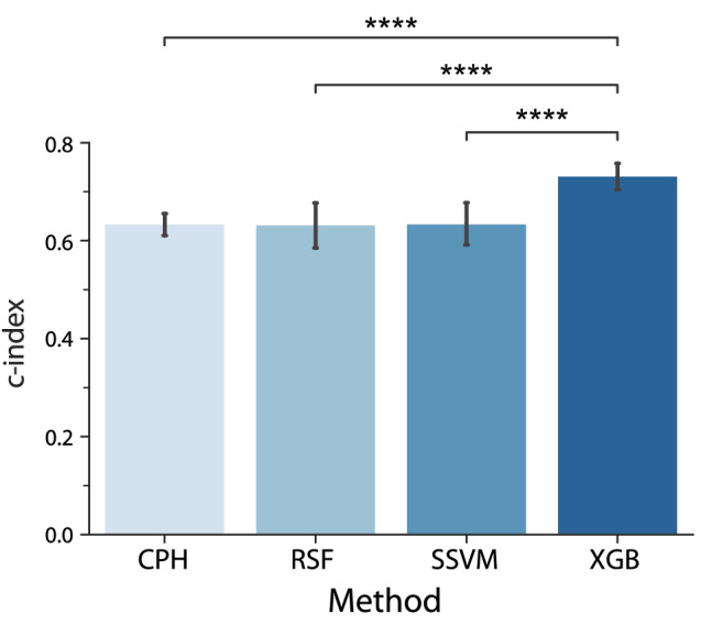
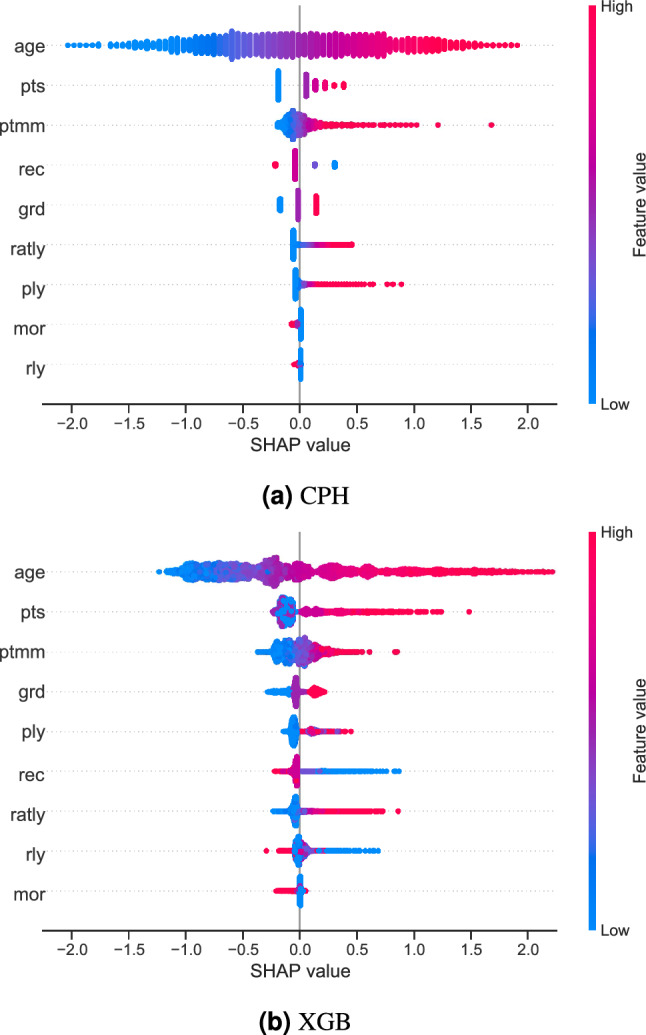
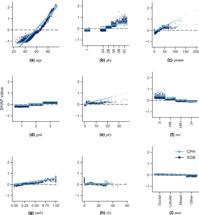
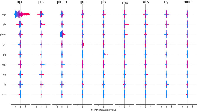
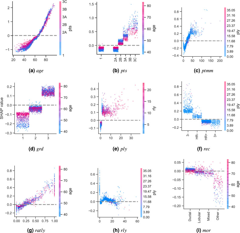
Cox Proportional Hazards (CPH) analysis is the standard for survival analysis in oncology. Recently, several machine learning (ML) techniques have been adapted for this task. Although they have shown to yield results at least as good as classical methods, they are often disregarded because of their lack of transparency and little to no explainability, which are key for their adoption in clinical settings. In this paper, we used data from the Netherlands Cancer Registry of 36,658 non-metastatic breast cancer patients to compare the performance of CPH with ML techniques (Random Survival Forests, Survival Support Vector Machines, and Extreme Gradient Boosting [XGB]) in predicting survival using the [Formula: see text]-index. We demonstrated that in our dataset, ML-based models can perform at least as good as the classical CPH regression ([Formula: see text]-index [Formula: see text]), and in the case of XGB even better ([Formula: see text]-index [Formula: see text]). Furthermore, we used Shapley Additive Explanation (SHAP) values to explain the models' predictions. We concluded that the difference in performance can be attributed to XGB's ability to model nonlinearities and complex interactions. We also investigated the impact of specific features on the models' predictions as well as their corresponding insights. Lastly, we showed that explainable ML can generate explicit knowledge of how models make their predictions, which is crucial in increasing the trust and adoption of innovative ML techniques in oncology and healthcare overall.

Figure 1

Average $c$-index of the different models using 10-fold cross-validation. Error bars represent 95% confidence intervals across folds. $\ast \ast \ast \ast p<0.0001$. All other comparisons were non-significant ($p>0.05$) and are not shown for the sake of clarity.

Figure 2

Summary plots for SHAP values. For each feature, one point corresponds to a single patient. A point’s position along the x axis (i.e., the actual SHAP value) represents the impact that feature had on the model’s output for that specific patient. Mathematically, this corresponds to the (logarithm of the) mortality risk relative across patients (i.e., a patient with a higher SHAP value has a higher mortality risk relative to a patient with a lower SHAP value). Features are arranged along the y axis based on their importance, which is given by the mean of their absolute Shapley values. The higher the feature is positioned in the plot, the more important it is for the model.

Figure 3

SHAP feature dependence plots. In the case of categorical variables, artificial jitter was added along the x axis to better show the density of the points. The scale of the y axis is the same for all plots in order to give a proper feeling of the magnitudes of the SHAP values for each feature (and therefore of their impact on the models’ output). In the case of the XGB model, the dispersion for each possible feature value along the y axis is due to interaction effects (which the CPH model is unable to capture).

Figure 4

SHAP interaction values. The main effect of each feature is shown in the diagonal, while interaction effects are shown off-diagonal.

Figure 5

SHAP feature dependence plots of the XGB model showing the largest interaction effect for each feature. In the case of categorical variables, artificial jitter was added along the x axis to better show the density of the points. In this case, the scale of the y axis is not the same for all plots in order to better appreciate the interaction effects.

References

1. Cox DR. Regression models and life-tables. J. R. Stat. Soc. Ser. B (Methodol.) 1972;34:187–202.
1. Wang P, Li Y, Reddy CK. Machine learning for survival analysis: A survey. ACM Comput. Surv. (CSUR) 2019;51:1–36. doi: 10.1145/3214306. - DOI
1. Mallett S, Royston P, Waters R, Dutton S, Altman DG. Reporting performance of prognostic models in cancer: A review. BMC Med. 2010;8:21. doi: 10.1186/1741-7015-8-21. - DOI - PMC - PubMed
1. Altman D, De Stavola B, Love S, Stepniewska K. Review of survival analyses published in cancer journals. Br. J. Cancer. 1995;72:511–518. doi: 10.1038/bjc.1995.364. - DOI - PMC - PubMed
1. Kourou K, Exarchos TP, Exarchos KP, Karamouzis MV, Fotiadis DI. Machine learning applications in cancer prognosis and prediction. Comput. Struct. Biotechnol. J. 2015;13:8–17. doi: 10.1016/j.csbj.2014.11.005. - DOI - PMC - PubMed