The importance of uncertainty quantification in model reproducibility

Abstract

Many computer models possess high-dimensional input spaces and substantial computational time to produce a single model evaluation. Although such models are often 'deterministic', these models suffer from a wide range of uncertainties. We argue that uncertainty quantification is crucial for computer model validation and reproducibility. We present a statistical framework, termed history matching, for performing global parameter search by comparing model output to the observed data. We employ Gaussian process (GP) emulators to produce fast predictions about model behaviour at the arbitrary input parameter settings allowing output uncertainty distributions to be calculated. History matching identifies sets of input parameters that give rise to acceptable matches between observed data and model output given our representation of uncertainties. Modellers could proceed by simulating computer models' outputs of interest at these identified parameter settings and producing a range of predictions. The variability in model results is crucial for inter-model comparison as well as model development. We illustrate the performance of emulation and history matching on a simple one-dimensional toy model and in application to a climate model. This article is part of the theme issue 'Reliability and reproducibility in computational science: implementing verification, validation and uncertainty quantification in silico'.

Keywords: Bayesian methods; emulation; error estimates.

Figure 1.

Schematic of the framework for analysing physical process y from computer model f and past physical data (observation) z and synthesizing all of the major uncertainties.

Figure 2.

Plot of (true) function f(x), x ∈ [ − 4, 3] (red line). The black dots represent the observed data at 6 equally spaced values of x. The solid line represent the emulator’s updated expectation E_F[f(x)], and the pair of blue dashed lines give the credible interval $E_{\text{F}}[f(\mathbf{\text{x}})]\pm 2\sqrt{{\text{Var}}_{\text{F}}[f(\mathbf{\text{x}})]}$, both as functions of x. (Online version in colour.)

Figure 3.

The model f(x) is given by the red line, the observed data z by the horizontal grey line. We include both observation error e (the grey dashed lines represent $z\pm 2\sqrt{\mathrm{Var}[\mathrm{e}]}$) and model discrepancy η (the red dashed lines show $f(\mathbf{\text{x}})\pm 2\sqrt{\mathrm{Var}[\eta ]}$). (Online version in colour.)

Figure 4.

(a) The emulator expectation and credible intervals as in figure 2; however, now the observation z plus observed error has been included as the horizontal grey solid and dashed lines respectively. The implausibilities $\mathcal{I}(x)$ are represented by the colours on the x-axis: red and green for high ($\mathcal{I}(x)>3$) and low ($\mathcal{I}(x)<3$) implausibility respectively, with the green interval defining the non-implausible region ${\mathcal{X}}_1$. (b) The second wave is performed by evaluating an additional point located within ${\mathcal{X}}_1$. The emulator becomes more accurate over ${\mathcal{X}}_1$ and the implausibility more strict, hence defining the smaller non-implausible region ${\mathcal{X}}_2$, given by the green interval. (Online version in colour.)

Figure 5.

Leave-One-Out diagnostics plots against each of the parameters for SANDU (top row) and ARMCU (second row) cases on original input scales. The predictions and two standard deviation prediction intervals are in black. The true model values are in green if they lie within two standard deviation prediction intervals, or red otherwise. The observation z plus observed error ($z\pm 2\sqrt{\text{Var}[e]}$) are shown by blue dashed lines. (Online version in colour.)

Figure 6.

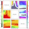
NROY density plots (upper triangle) and minimum implausibility plots (lower triangle). Each panel plots either NROY density or minimum implausibility for a pair of parameters. NROY densities, for each pixel on any panel in the upper triangle, represent the proportion of points in the input space behind that pixel that are NROY and are indicated by the colour whose scale is indicated on the right. Grey coloured regions are completely ruled out. Minimum implausibilities, for each pixel on any panel on the lower triangle of the picture, represent the smallest implausibilities found in input space. These plots are oriented the same way as those on the upper triangle, for the ease of visual comparison. Currently used parameter values in GCM is depicted as the square on the NROY density plots and as the circular point on the minimum implausibility plots. (Online version in colour.)

References

1. Goldstein M. 2006. Subjective Bayesian analysis: principles and practice. Bayesian Anal. 1, 403–420. ( 10.1214/06-BA116) - DOI
1. Vernon I, Goldstein M, Bower R. 2014. Galaxy formation: Bayesian history matching for the observable universe. Stat. Sci. 29, 81–90. ( 10.1214/12-STS412) - DOI
1. Gettelman A, Rood RB. 2016. Demystifying climate models. A Users Guide to Earth System Models.
1. Hourdin F et al. 2017. The art and science of climate model tuning. Bull. Am. Meteorol. Soc. 98, 589–602. ( 10.1175/BAMS-D-15-00135.1) - DOI
1. WCRP. Coupled Model Intercomparison Project (CMIP). https://www.wcrp-climate.org/wgcm-cmip, 2020. (accessed 22 May 2020).
LinkOut - more resources