The genetic architecture of human complex phenotypes is modulated by linkage disequilibrium and heterozygosity

Abstract

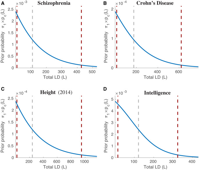
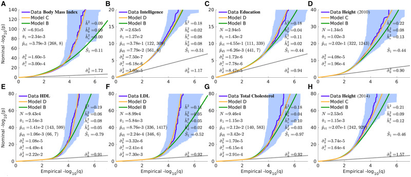
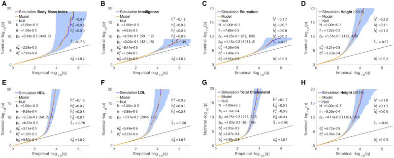
We propose an extended Gaussian mixture model for the distribution of causal effects of common single nucleotide polymorphisms (SNPs) for human complex phenotypes that depends on linkage disequilibrium (LD) and heterozygosity (H), while also allowing for independent components for small and large effects. Using a precise methodology showing how genome-wide association studies (GWASs) summary statistics (z-scores) arise through LD with underlying causal SNPs, we applied the model to GWAS of multiple human phenotypes. Our findings indicated that causal effects are distributed with dependence on total LD and H, whereby SNPs with lower total LD and H are more likely to be causal with larger effects; this dependence is consistent with models of the influence of negative pressure from natural selection. Compared with the basic Gaussian mixture model it is built on, the extended model-primarily through quantification of selection pressure-reproduces with greater accuracy the empirical distributions of z-scores, thus providing better estimates of genetic quantities, such as polygenicity and heritability, that arise from the distribution of causal effects.

Keywords: effect size; heritability; linkage disequilibrium; minor allele frequency; natural selection; polygenicity.

Figure 1

Examples of ${\pi }_1\times$ prior probability functions $p_c(L)$ used in Equations (4) and (5), where L is reference SNP total LD (see Equation (3) for the general expression, and Appendix Table G for parameter values). These functions can be summarized by three quantities: the maximum value, $p_{c1}$, which occurs at L = 1; the total LD value, L = m_c, where $p_c(m_c)=p_{c1}/2$, given by the gray dashed lines in the figure; and the total LD width of the transition region, w_c, defined as the distance between where $p_c(L)$ falls to 95% and 5% of $p_{c1}$ given by the flanking red dashed lines in the figure. Numerical values of $p_{c1}$, m_c, and w_c are given in Table 1 and Figures 2 and 3. $p_d(L)$ is similar. Plots of $p_c(L)$ and $p_d(L)$, where relevant, for all phenotypes are shown in Supplementary Figures S3–S5.

Figure 2

QQ plots of (pruned) z-scores for qualitative phenotypes (dark blue, 95% confidence interval in light blue) with model prediction (yellow): (A) Alzheimer’s Disease, excluding chromosome 19; (B) Amyotrophic Lateral Sclerosis, chromosome 9 only; (C) Bipolar Disorder; (D) Schizophrenia; (E) AD, chromosome 19 only; (F) Crohn’s Disease; (G) Ulcerative Colitis; and (H) Coronary Artery Disease. See Supplementary Figures S15–S22. amplitude of the full $p_c(L)$ function, which occurs at L = 1; the values (m_c, w_c) in parentheses following it are the total LD (m_c) where the function falls to half its amplitude (the middle gray dashed lines in Figure 1 are examples), and the total LD width (w_c) of the transition region (distance between flanking red dashed lines in Figure 1). Similarly for $p_{d1} (m_d,w_d)$, where given. $h_b^2,\hspace{0.17em}{h}_c^2$, and $h_d^2$ are the heritabilities associated with the “b,” “c,” and “d” Gaussians, respectively. h² is the total SNP heritability, reexpressed as $h_l^2$ on the liability scale for binary phenotypes. Parameter values are also given in Table 1 and heritabilities are also in Table 3; numbers of causal SNPs are in Table 2. Reading the plots: on the vertical axis, choose a P-value threshold for typed or imputed SNPs (SNPs with z-scores; more extreme values are further from the origin), then the horizontal axis gives the proportion, q, of typed SNPs exceeding that threshold (higher proportions are closer to the origin). See also Supplementary Figure S1, where the y-axis is restricted to $0\le -{\hspace{0.17em}\text{log}\hspace{0.17em}}_{10}(p)⩽10$. The $h_b^2$ values reported here are from one component in the extended model; values for the exclusive basic model are reported as $h_{\beta }^2$ in Holland et al. (2020).

Figure 3

QQ plots of (pruned) z-scores for quantitative phenotypes (dark blue, 95% confidence interval in light blue) with model prediction (yellow): (A) Body Mass Index; (B) Intelligence; (C) Education; (D) Height (2010); (E) High-density Lipoprotein; (F) Low-density Lipoprotein; (G) Total Cholesterol; and (H) Height (2014). See Supplementary Figures S23–S29. For HDL, $p_c(L)=p_{c1}$ for all L; for bipolar disorder and LDL, $p_d(L)=p_{d1}$ for all L. See caption to Figure 2 for further description. See also Supplementary Figure S2, where the y-axis is restricted to $0\le -{\hspace{0.17em}\text{log}\hspace{0.17em}}_{10}(p)⩽10$. For (A) BMI, see also Supplementary Figure S37.

Figure 4

A 4 × 4 subset from a 10 × 10 heterozygosity × TLD grid of QQ plots for HDL; see Figure 3E for the overall summary plot. Similar plots for all phenotypes are in Supplementary Figures S15–S29. The light gray curves are 95% confidence intervals for the data; ${\widehat{\lambda }}_D$ and ${\widehat{\lambda }}_M$ are the “genomic inflation factors” calculated from the QQ subplots, for the data and the model prediction, respectively; n is the number of SNPs; H is heterozygosity, L is total LD, and the square brackets give their ranges for GWAS SNPs in each grid element.

Figure 5

Model results for height (2014) using the BC model. The reference panel SNPs are binned with respect to both heterozygosity (H) and total LD (L) in a 50 × 50 grid for $0.02\le H⩽0.5$ and $1\le L⩽500$. Shown are model estimates of: (A) ${\hspace{0.17em}\text{log}\hspace{0.17em}}_{10}$ of the percentage of heritability in each grid element; (B) for each element, the average heritability per causal-SNP in the element; (C) ${\hspace{0.17em}\text{log}\hspace{0.17em}}_{10}$ of the number of causal SNPs in each element; and (D) the expected ${\beta }^2$ for the element-wise causal SNPs. Note that H increases from top to bottom.

Figure 6

QQ plots of (pruned) z-scores for simulated qualitative phenotypes (dark blue, 95% confidence interval in light blue) with model prediction (yellow). See Figure 2. The value given for $p_{c1}$ is the amplitude of the full $p_c(L)$ function, which occurs at L = 1; the values (m_c, w_c) in parentheses following it are the total LD (m_c) where the function falls to half its amplitude (the middle gray dashed lines in Figure 1 are examples), and the total LD width (w_c) of the transition region (distance between flanking red dashed lines in Figure 1). Similarly for $p_{d1} (m_d,w_d)$, where given. $h_b^2,\hspace{0.17em}{h}_c^2$, and $h_d^2$ are the heritabilities associated with the “b,” “c,” and “d” Gaussians, respectively. h² is the total SNP heritability, re-expressed as $h_l^2$ on the liability scale for binary phenotypes. Reading the plots: on the vertical axis, choose a p-value threshold for typed SNPs (SNPs with z-scores; more extreme values are further from the origin), then the horizontal axis gives the proportion, q, of typed SNPs exceeding that threshold (higher proportions are closer to the origin). See Appendix Tables C1 and C2 for a comparison of numerical values between model estimates for real phenotypes and Hapgen-based simulations where the underlying distributions of simulation causal effects were given based on the real phenotype model parameters (with ${\sigma }_0=1$).

Figure 7

QQ plots of (pruned) z-scores for simulated quantitative phenotypes (dark blue, 95% confidence interval in light blue) with model prediction (yellow). See Figure 3. See caption to Figure 2 for further description. See Appendix Tables C1 and C2 for a comparison of numerical values between model estimates for real phenotypes and Hapgen-based simulations where the underlying distributions of simulation causal effects were given based on the real phenotype model parameters (with ${\sigma }_0=1$).

References

1. Al-Chalabi A, Fang F, Hanby MF, Leigh PN, Shaw CE, et al.2010. An estimate of amyotrophic lateral sclerosis heritability using twin data. J Neurol Neurosurg Psychiatry 81:1324–1326. - PMC - PubMed
1. Alzheimer’s Association. 2018. 2018 Alzheimer’s disease facts and figures. Alzheimer’s Dementia, 14:367–429. - PubMed
1. Berg JJ, Harpak A, Sinnott-Armstrong N, Joergensen AM, Mostafavi H, et al.2019. Reduced signal for polygenic adaptation of height in UK biobank. eLife. 8:e39725. - PMC - PubMed
1. Bulik-Sullivan BK, Loh P-R, Finucane HK, Ripke S, Yang J, Schizophrenia Working Group of the Psychiatric Genomics Consortium, et al.2015. LD score regression distinguishes confounding from polygenicity in genome-wide association studies. Nat Genet. 47:291–295. - PMC - PubMed
1. Burisch J, Jess T, Martinato M, Lakatos PL, ECCO EpiCom.. 2013. The burden of inflammatory bowel disease in Europe. J Crohns Colitis. 7:322–337. - PubMed
Publication types