Computational modelling of muscle fibre operating ranges in the hindlimb of a small ground bird (Eudromia elegans), with implications for modelling locomotion in extinct species

Abstract

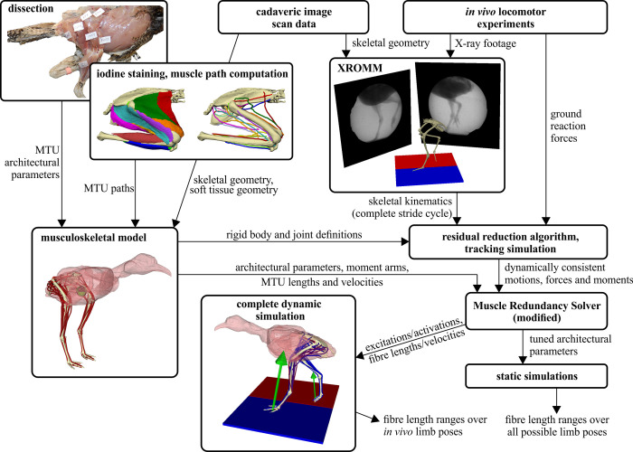
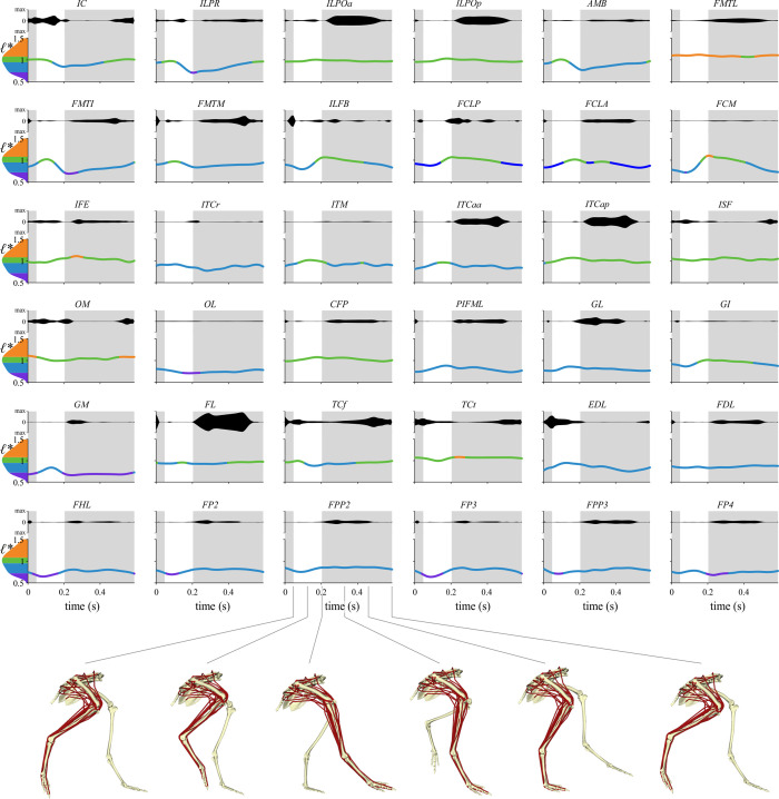
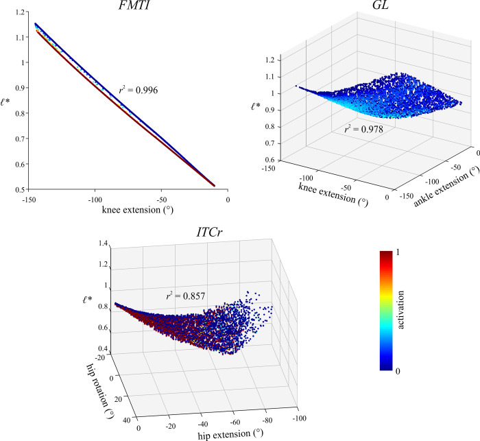
The arrangement and physiology of muscle fibres can strongly influence musculoskeletal function and whole-organismal performance. However, experimental investigation of muscle function during in vivo activity is typically limited to relatively few muscles in a given system. Computational models and simulations of the musculoskeletal system can partly overcome these limitations, by exploring the dynamics of muscles, tendons and other tissues in a robust and quantitative fashion. Here, a high-fidelity, 26-degree-of-freedom musculoskeletal model was developed of the hindlimb of a small ground bird, the elegant-crested tinamou (Eudromia elegans, ~550 g), including all the major muscles of the limb (36 actuators per leg). The model was integrated with biplanar fluoroscopy (XROMM) and forceplate data for walking and running, where dynamic optimization was used to estimate muscle excitations and fibre length changes throughout both gaits. Following this, a series of static simulations over the total range of physiological limb postures were performed, to circumscribe the bounds of possible variation in fibre length. During gait, fibre lengths for all muscles remained between 0.5 to 1.21 times optimal fibre length, but operated mostly on the ascending limb and plateau of the active force-length curve, a result that parallels previous experimental findings for birds, humans and other species. However, the ranges of fibre length varied considerably among individual muscles, especially when considered across the total possible range of joint excursion. Net length change of muscle-tendon units was mostly less than optimal fibre length, sometimes markedly so, suggesting that approaches that use muscle-tendon length change to estimate optimal fibre length in extinct species are likely underestimating this important parameter for many muscles. The results of this study clarify and broaden understanding of muscle function in extant animals, and can help refine approaches used to study extinct species.

Fig 1. Schematic overview summarizing the workflow of the study.

The input data are anatomical measurements of muscles and bones (obtained by physical and digital means) and in vivo experimental data; the outputs are a high-fidelity computational musculoskeletal model, estimations of in vivo muscle function, and estimations of the range of viable operating lengths of each muscle. XROMM, X-ray reconstruction of moving morphology; MTU, muscle–tendon unit.

Fig 2. Musculoskeletal model of the tinamou.

(A) Rigid body mechanics component of the model, shown in the neutral pose used in this study; the green and black sphere denotes the whole-body centre of mass in this pose. Scale bar refers to this panel. (B) Skeleton and joints shown collapsed in the XROMM neutral pose [91], which differs from the neutral pose of the musculoskeletal model by offsets of 90° or 180° about the flexion–extension axes. In both A and B, anatomical coordinate systems used to define joint coordinate systems are illustrated; blue (z-axis) corresponds to flexion–extension, green (y-axis) corresponds to abduction–adduction and red (x-axis) corresponds to long-axis rotation. (C, D) The 36 muscle–tendon actuators for the right leg, shown for an arbitrary standing posture in lateral (C) and anterior (D) views. (E–G) Close-ups on different parts of the model to show the actuator paths used to model muscle–tendon units, along with various wrapping surfaces (blue and purple geometries) used to help constrain these paths. (H) A single contact sphere was applied to the digits (terminal) segment of each limb, with radius and location as shown.

Fig 3. Tuning factors used in the optimal solution for the inverse simulation.

These factors are multiplied against the original assigned values for optimal fibre length (ℓ_o) and tendon slack length (L_S) to derive the tuned parameters for each MTU.

Fig 4. Reserve actuator contributions to external joint moments.

This is shown for walking (A) and running (B) trials. Grey regions denote the stance phase, white regions denote the swing phase. Note the strong contributions to external joint moment made by reserves acting about the abduction–adduction and long-axis rotation DOFs of the knee and ankle joints. Also illustrated are the kinematics of the left hindlimb (reversed for visualization) at various parts of the stride cycle.

Fig 5. Time histories of muscle excitation and fibre length change for each MTU in the walking simulation.

Excitations (from zero recruitment to possible maximal recruitment) are plotted above normalized fibre lengths for each MTU, the latter of which are colour coded according to where on the active force–length curve fibres are operating: purple = steep ascending limb, blue = shallow ascending limb, green = plateau, orange = descending limb (divisions approximately correspond to those of Arnold and Delp [15]). Excitation profiles obtained in the simulation are reflected about the abscissa so as to visually emulate the appearance of experimental EMG signals. Grey regions denote the stance phase, white regions denote the swing phase. See Table 2 for muscle abbreviations.

Fig 6. Time histories of muscle excitation and fibre length change for each MTU in the running simulation.

Formatting is the same as for Fig 5.

Fig 7. Comparison of exemplar outputs for excitation and fibre length change in the running simulation against previous experimental data (electromyography and sonomicrometry), for validation of the modelling and simulation approach.

For each muscle, experimental data are shown in blue, and simulation outputs are shown in red; in some studies sonomicrometry data were reported in absolute terms, whereas in others it was reported in relative terms. See Table 2 for muscle abbreviations. Fibre length data do not exist for the AMB or ILFB. Experimental results were digitized from the original studies and scaled according to swing and stance phase durations. Sources of experimental data are as follows: ILPOp, guineafowl running at 2.5 m/s [9]; FCLP and FCLA, guineafowl running at 1.5 m/s [38]; GL, guineafowl running at 1.3 m/s [36]; GM, guineafowl running at 2 m/s [141]; FP4, guineafowl running at 1.3 m/s [36]; AMB and ILFB, guineafowl running at 1 m/s [27].

Fig 8. Distribution of normalized fibre lengths for each MTU in static simulation 1 (3,827 viable poses).

Each distribution is visualized as a histogram (intervals of 0.02× ℓ_o), the vertical axis of which is scaled by the magnitude (number of counts) of the most frequent bin. Colours signify the various parts of the active force–length curve as per Figs 5 and 6. Also shown are the ranges of normalized fibre lengths used in vivo during walking (grey bars) and running (white bars). Instances where the minimum or maximum normalized fibre length achieved reached below 0.5 or above 1.5 (respectively) are indicated. The very small range recovered for the FMTL is due to the way its path was represented in the musculoskeletal model, crossing over the lateral femoral condyle close to the flexion–extension axis of the knee, such that it had little opportunity to undergo change in MTU length in the first instance. Similarly, the small range recovered for the ILPOa likewise reflects its path in the model passing close to the flexion–extension axes of the hip and knee. See Table 2 for muscle abbreviations.

Fig 9. Ranges of normalized fibre lengths and MTU lengths across all viable limb poses.

The results illustrated here are for static simulation 1, but a very similar pattern was achieved for the other three simulations as well. (A) Range of normalized fibre length compared to range of MTU length (normalized by optimal fibre length) for each MTU; all points plot on or below the line of parity, with the most extreme outliers indicated (see Table 2 for abbreviations). (B) Ratio of MTU length range to fibre length range compared to pennation angle. As fibre length range can at most be equal to MTU length range, this ratio is one or less; the lower it is (i.e., the further a point plots further from the line or parity in A), the greater the discrepancy between length changes at the level of the MTU and fibre. A higher pennation angle leads to a greater decoupling between changes in fibre and MTU lengths. (C) Ratio of MTU length range to fibre length range compared to relative tendon length, expressed as the ratio of slack to fibre length. A relatively longer tendon leads to a greater decoupling between changes in fibre and MTU lengths. In all panels, points are colour coded by the order of muscles as listed in Table 2, which are arranged in a proximal-to-distal fashion.

Fig 10. Exemplar plots illustrating variation in normalized fibre length with respect to joint angle(s) in the static simulations, shown here for the combined results of simulations 1 and 2.

The FMTI actuates one DOF, the GL actuates two DOFs and the ITCr actuates three DOFs (only two of which are plotted here; hip abduction omitted for clarity). The coefficient of determination for a hyperplane fit is also given in each case. See Table 2 for muscle abbreviations.

References

-
- McMahon TA (1984) Muscles, Reflexes, and Locomotion. Princeton: Princeton University Press.
- May MT (1968) Galen: On the Usefulness of the Parts of the Body. New York: Cornell University Press.
- Hill AV (1938) The heat of shortening and the dynamic constants of muscle. Proceedings of the Royal Society of London, Series B 126: 136–195. - PubMed
- Zajac FE (1989) Muscle and tendon: properties, models, scaling, and application to biomechanics and motor control. Critical Reviews in Biomedical Engineering 17: 359–410. - PubMed
Publication types
MeSH terms
LinkOut - more resources
Full Text Sources
Other Literature Sources