A Review of Recent Distributed Optical Fiber Sensors Applications for Civil Engineering Structural Health Monitoring

Abstract

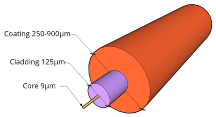
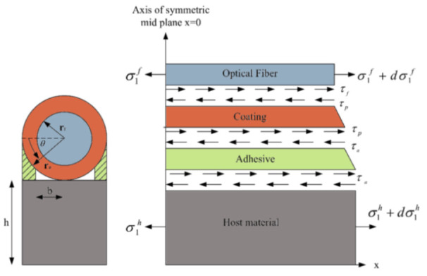
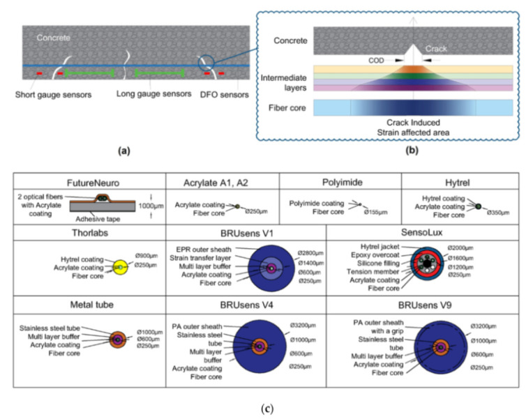
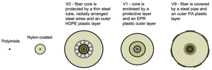
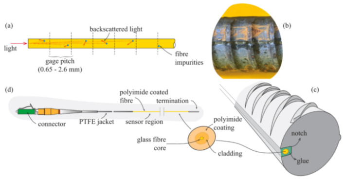
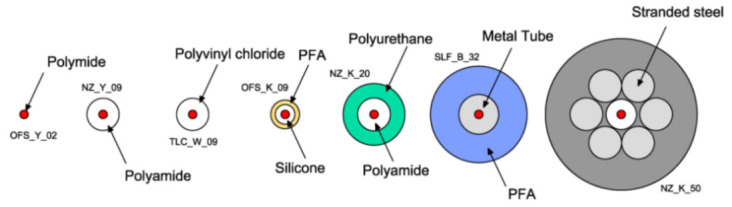
The present work is a comprehensive collection of recently published research articles on Structural Health Monitoring (SHM) campaigns performed by means of Distributed Optical Fiber Sensors (DOFS). The latter are cutting-edge strain, temperature and vibration monitoring tools with a large potential pool, namely their minimal intrusiveness, accuracy, ease of deployment and more. Its most state-of-the-art feature, though, is the ability to perform measurements with very small spatial resolutions (as small as 0.63 mm). This review article intends to introduce, inform and advise the readers on various DOFS deployment methodologies for the assessment of the residual ability of a structure to continue serving its intended purpose. By collecting in a single place these recent efforts, advancements and findings, the authors intend to contribute to the goal of collective growth towards an efficient SHM. The current work is structured in a manner that allows for the single consultation of any specific DOFS application field, i.e., laboratory experimentation, the built environment (bridges, buildings, roads, etc.), geotechnical constructions, tunnels, pipelines and wind turbines. Beforehand, a brief section was constructed around the recent progress on the study of the strain transfer mechanisms occurring in the multi-layered sensing system inherent to any DOFS deployment (different kinds of fiber claddings, coatings and bonding adhesives). Finally, a section is also dedicated to ideas and concepts for those novel DOFS applications which may very well represent the future of SHM.

Keywords: DFOS; DOFS; SHM; distributed monitoring; distributed optical fiber sensors; distributed sensing; review; structural health monitoring.

Figure 1

3D illustration of an optical fiber cross-section.

Figure 2

Growth of Optical Fiber Sensors (OFS) technological market [36].

Figure 3

(a) Distributed OFS (DOFS) fiber and (b) ODiSI-6000 model Optical Backscatter Reflectometer (OBR) interrogator manufactured by LUNA Technologies.

Figure 4

Free body diagram for the symmetrical section of the optical fiber and the substrates together with their relative shear transfer (adapted from [40]).

Figure 5

Crack detection using DOFS techniques: (a) Comparison of the traditional sensors, (b) strain transferring between layers and (c) the tested cables (adapted from [44]).

Figure 6

Test setup: three-dimensional specimen detailing and photography [48].

Figure 7

Strain profiles of a 15 × 15 × 210 mm Ø20 Reinforced Concrete (RC) tie test with the DOFS bonded with a combination of groove, cyanoacrylate and silicone [49].

Figure 8

Influence of the rib pattern on the steel strain profiles during the double pull-out test of the RC tie 15 × 15 × 240 mm Ø20 (top five figures). Relative average reading noise (bottom) [49].

Figure 9

Total amount of anomalistic readings grouped per bonding technique [49].

Figure 10

Finite element mesh of (a) the 3D geometry and (b) the cross-sectional view of the system [42].

Figure 11

Strain profiles recorded by DOFS bonded to the concrete specimen with three soft adhesives (Bi-component epoxy, Mastic silicone and Silicone rubber) [42].

Figure 12

Crack locations and openings, steel stresses and forces in front layers of stirrups for Panel 1 at (a) 80 kN and (b) 110 kN as well as for Panel 2 at (c) 90 kN and (d) 150 kN [54].

Figure 13

Multiple strain profiles from the DOFS where the red triangular makers indicate the determined crack position based on the strain profile at maximum load and the grey shaded area correspond to position determined from the Digital Image Correlation (DIC) [59].

Figure 14

Comparison between the crack width measured by the DIC and calculated from the DOFS measurements [59].

Figure 15

Installation of the DOFS: (a) installation of robust DOFS cable in a reinforcement bar by inserting it into a previously milled groove; (b) comparison of thin and robust DOFS; (c) installation of thin DOFS on the surface of a reinforcement bar by bonding it with cyanoacrylate adhesive and protecting it with silicone; (d) installation of robust DOFS on the surface of a reinforcement bar by mechanically anchoring the cable to the reinforcement with electric tape; (e) multi-layer configuration of embedded DOFS in the beam specimens and (f) loading setup and DOFS installation configuration for the RC beam specimens (adapted from [60]).

Figure 16

Real cracking pattern and obtained with DOFS in two different beams (adapted from [64]).

Figure 17

DOFS cables used in [66].

Figure 18

DOFS-integrating DIC strain distributions at different load steps [68].

Figure 19

Strain along the bottom reinforcement during cycling for four deep beam specimens [69].

Figure 20

Ultra Sonics (US) and DOFS sensors attached to the rebars before casting of concrete [71].

Figure 21

(a) Tested RC ties’ with their respective bonding technologies, with (c) and without (b) the addition of a protective silicone layer. The DOFS-instrumented rebars were monitored by means of an (d) ODiSI-A OBR interrogator [77].

Figure 22

(a) Back-scattering mechanism due to fiber core impurities, (b) view of the fiber-optic sensor glued to a steel rebar, (c) sketch of the fiber optical cable placed in the groove and adhering to the steel due to two-component glue and (d) description of the fiber optic cable structure with angle polished connector on one side and termination (which avoids light reflection) on the opposite [78].

Figure 23

Tensile tests—specimen TC04: (a) cracking pattern in the cyclic loading phase, (b) stress-strain relationship for all cycles (in grey) and cycle #6 (in green) indicating load levels, (c) profiles of stresses, calculated on the basis of the measured DOFS (here defined as FOM) strains and (d) bond stresses τ profiles along the steel rebar (adapted from [78]).

Figure 24

DOFS cables used in [79].

Figure 25

Specimen failure due to punching shear and its crack pattern [86].

Figure 26

Slab 3-C-45 DOFS strains: (a) 50 kN, (b) 100 kN, (c) 150 kN (adapted from [86]).

Figure 27

Test setup: (a) instrumented test slab, (b) testing with surrounding insulation [88].

Figure 28

Fiber arrangement for the Timber–Concrete Composite (TCC) slab monitoring [89].

Figure 29

(a) Specimen’s cross-sectional layout and (b) comparison of the nylon bottom DOFS measured strains between a non-corroded control beam (BS-C) versus a corroded one (BS-01) for three applied load steps, 20 kN, 60 kN and 100 kN (adapted from [90]).

Figure 30

Photograph of the DOFS deployment on the steel bars: (a) Reference bar (b) L4 longitudinal deployment, (c) S0 spacing 0 mm, (d) S2 spacing 2 mm, (e) S5 spacing 5 mm and (f) S10 spacing 10 mm [93].

Figure 31

(a) Photography of the tested specimen and (b) cut section along the steel corroded bar [23].

Figure 32

Applications of DOFS in structural fire testing of: (a) Steel beam and (b) RC beams [96].

Figure 33

Positioning of the optical fiber on the textile reinforcement [98].

Figure 34

(a) Damage status at 0.15% drift, (b–d) are the strain profiles measured in the top fibers A, B and C at drift levels below 0.15% and (e) picture of the cracked specimen (adapted from [100]).

Figure 35

Experimental test setup (adapted from [101]).

Figure 36

2D spatial strain distribution in the: (a) vertical and (b) horizontal directions [101].

Figure 37

Nine Wells Bridge [107].

Figure 38

Beam cross section showing the fiber-optic cable locations: (a) illustration and (b) photograph (adapted from [107]).

Figure 39

(a) DOFS deployment layout and (b) prestressed concrete beam cross-sections—edge TYE7 beams (left) and internal TY7 beams (right) [110].

Figure 40

(a) General scheme of DOFS monitoring and (b) its photograph inside the box girder (adapted from [111]).

Figure 41

(a) A 3D sketch and (b) a cross-section of the DOFS deployment layout for temperature measurements in the study case pile cap [20].

Figure 42

Temperature variation as a function of the DOFS coordinates specified in Figure 41 [20].

Figure 43

(a) Location of the instrumented columns and walls and (b) DOFS tied to the reinforcement prior to concreting [114].

Figure 44

The total cumulative axial displacement (negative = shortening) of the instrumented columns C8 and wall W1 measured at the mid-height of every level during the first 12 months of construction (adapted from [114]).

Figure 44

The total cumulative axial displacement (negative = shortening) of the instrumented columns C8 and wall W1 measured at the mid-height of every level during the first 12 months of construction (adapted from [114]).

Figure 45

(a) Photograph of the DOFS cables, (b) an illustration of their cross-sections and (c) of their designed installation position and finally (d) photography of the deployment process (adapted from [119]).

Figure 46

Strains measured along the sensors when the study case airplane rear landing gear was rolled on them [119].

Figure 47

Installation of fiber on rail [120].

Figure 48

DOFS-sampled strains for three different hi-rail vehicle positions along the track (adapted from [120]).

Figure 49

Measurement schemes for concrete piles: (a) spot, (b) quasi-continuous, (c) distributed [123].

Figure 50

Installation of the DOFS and the pile [7].

Figure 51

Typical cross-section layout of DOFS cables attached to (a) a steel pile and to (b) a steel cage; photography of the latter is represented in (c) (adapted from [124]).

Figure 52

Distribution of strains along individual DOFS (a) after the driving of a steel pile (b) during a static load testing of the CFA pile and (c) the crack evolution inside a precast concrete pile (adapted from [124]).

Figure 53

(a) Changes in strains along the pile during Bi-Directional Static Load Test (BDSLT) and (b) the calculated load distribution along it (adapted from [125]).

Figure 54

Fiber optic deployment layout in the study case bored pile [126]. (a) Total view;(b) Cross section I-I; (c) Enlarged view.

Figure 55

(a) Monitoring area plan and (b) resulting strains (adapted from [128]).

Figure 56

Illustration of soil subsidence and DOFS vertical deployment in a borehole as performed in [131].

Figure 57

Monitoring chart and site map of pipeline trench collapse accident [133].

Figure 58

Different kinds of anchors used in the test from top to bottom: V1 tube-anchored cable, V2 aluminum block anchored cable, V3 smooth cable [132].

Figure 59

DOFS installation by means of plastic hooks for coupling the DOFS in an anchor’s (a) extremity bar and (b) internal bar [139].

Figure 60

Schematic representation of single borehole with multiple anchors and with two DOFS deployed along the tendons of each individual anchor. Two fiber loops were also deployed in the grout material [140].

Figure 61

(a) Three fiber optic-instrumented soil nails at a construction site and (b) their cable layout [140].

Figure 62

Geotechnical sensors (in blue) and fiber optics cable (in red) on the western (a) and southern-eastern (b) sides of the buttress [142].

Figure 63

DOFS installation system inside the tunnel lining: (a) Schematic representation and (b) practical realization [147].

Figure 64

Measured strain distribution at the rock-side layer in peripheral direction: (a) 12 h after installation at top-heading, (b) 48 h after installation at top-heading, (c) 12 h after installation at invert and (d) 48 h after installation at invert [147].

Figure 65

(a) Tunnel and distributed temperature and strain system layout and (b) optical fiber implementation on iron bars of the braced girder of the primary lining [146].

Figure 66

Monitored tunnel section [150].

Figure 67

Hoop strain nephogram when the pipe was corroded at 200 h (a) 2D and (b) 3D and wall thickness nephogram when the pipe was corroded at 200 h. (c) 2D and (d) 3D. [158].

Figure 68

(a) Schematic illustration of the fiber helical wrapping around the pipe segments and (b) photo of one of the pipe’s side adapters [159].

Figure 69

(a) Study case offshore turbine (b) DOFS bonded with epoxy to the sample pile (adapted from [26]).

Figure 70

Strain values per corresponding elevation from 0 kN to 900 kN [26].

Figure 71

Submarine cable map in 2015 [166].

Figure 72

(a) Spectrogram of the seismic signal measured by a reference seismograph (b) Spectrogram of the DAS data denoised with a 2D linear bandpass filter and a (c) Spectrogram of the DAS data denoised with a 1D adaptive LMS filter (adapted from [28]).

Figure 73

(a) Fiber Bragg Grating (FBG)-based acceleration sensor and (b) Distributed Optical Fiber Vibration Sensor [52].

Figure 74

DOFS extracted strain evolution in time: (a) before post-processing and (b) after post-processing with PICM—Polynomial Interpolation Comparison Method.

References

1. Barrias A., Casas J.R., Villalba S. A Review of Distributed Optical Fiber Sensors for Civil Engineering Applications. Sensors. 2016;16:748. doi: 10.3390/s16050748. - DOI - PMC - PubMed
1. Brownjohn J.M.W. Structural health monitoring of civil infrastructure. J. Philosofical Trans. A Math. Phys. Eng. Sci. 2006;365:589–622. doi: 10.1098/rsta.2006.1925. - DOI - PubMed
1. Housner G.W., Bergman L.A., Caughey T.K., Chassiakos A.G., Claus R.O., Masri S.F., Skelton R.E., Soong T.T., Spencer B.F., Yao J.T.P. Structural control: Past, present and future. J. Eng. Mech. 1997;123:897–971. doi: 10.1061/(ASCE)0733-9399(1997)123:9(897). - DOI
1. Cawley P. Structural health monitoring: Closing the gap between research and industrial deployment. Struct. Health Monit. 2018;17:1225–1244. doi: 10.1177/1475921717750047. - DOI
1. Baker M. Sensors Power Next-Generation SHM. [(accessed on 20 October 2020)]; Available online: https://www.sensorland.com/HowPage131.html.
LinkOut - more resources