Granular layEr Simulator: Design and Multi-GPU Simulation of the Cerebellar Granular Layer

Abstract

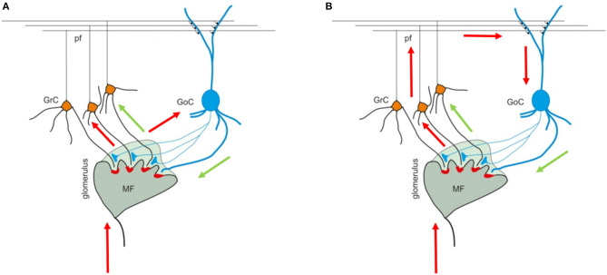
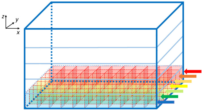
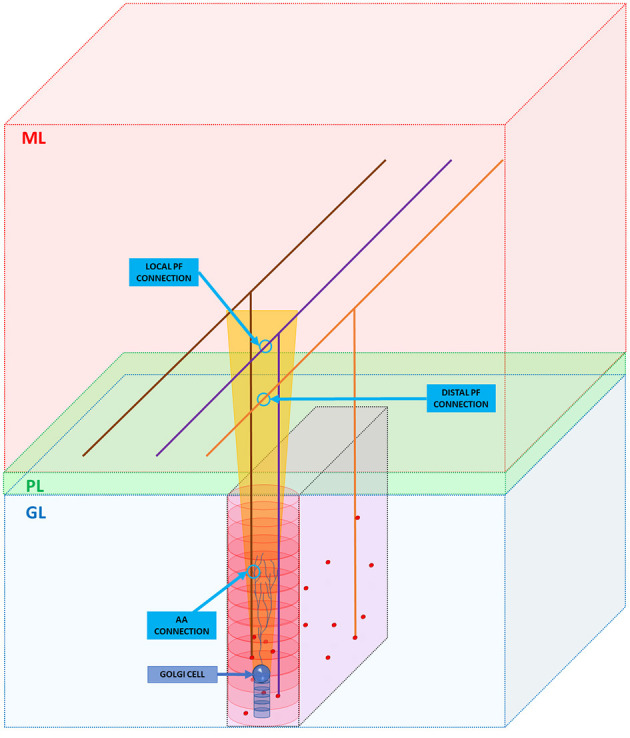
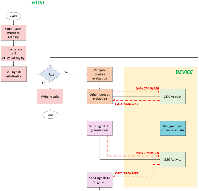
In modern computational modeling, neuroscientists need to reproduce long-lasting activity of large-scale networks, where neurons are described by highly complex mathematical models. These aspects strongly increase the computational load of the simulations, which can be efficiently performed by exploiting parallel systems to reduce the processing times. Graphics Processing Unit (GPU) devices meet this need providing on desktop High Performance Computing. In this work, authors describe a novel Granular layEr Simulator development implemented on a multi-GPU system capable of reconstructing the cerebellar granular layer in a 3D space and reproducing its neuronal activity. The reconstruction is characterized by a high level of novelty and realism considering axonal/dendritic field geometries, oriented in the 3D space, and following convergence/divergence rates provided in literature. Neurons are modeled using Hodgkin and Huxley representations. The network is validated by reproducing typical behaviors which are well-documented in the literature, such as the center-surround organization. The reconstruction of a network, whose volume is 600 × 150 × 1,200 μm³ with 432,000 granules, 972 Golgi cells, 32,399 glomeruli, and 4,051 mossy fibers, takes 235 s on an Intel i9 processor. The 10 s activity reproduction takes only 4.34 and 3.37 h exploiting a single and multi-GPU desktop system (with one or two NVIDIA RTX 2080 GPU, respectively). Moreover, the code takes only 3.52 and 2.44 h if run on one or two NVIDIA V100 GPU, respectively. The relevant speedups reached (up to ~38× in the single-GPU version, and ~55× in the multi-GPU) clearly demonstrate that the GPU technology is highly suitable for realistic large network simulations.

Keywords: computational modeling; granular layer simulator; graphics processing unit; high performance computing; neuroscience; parallel processing.

Figure 1

Cerebellar granular layer. (A) The granular layer circuit receives the input from the mossy fibers (MFs) that reach the glomeruli (GLOs). Here, they reach and excite the Golgi cells (GOCs) and granules (GRCs) dendrites. Once the GRCs are stimulated, the signal travels along the GRCs ascending axon and parallel fibers (PFs) and, then, can reach the GOCs apical dendrites (feedback loop). (B) On the other hand, the MFs signals reach the GOCs cells that inhibit the GRCs (feedforward loop). The black arrows indicate the direction of the signals in the loops. The image is taken from Mapelli et al. (2014).

Figure 2

Volume division for the displacement of the GOCs. The volume is divided into z-layers (five in this image). Each z-layer (x-y plane) is divided into rows along the y-axis (indicated with the arrows), where rectangular parallelepipeds are placed to host the cells. The algorithm starts placing the neurons from the blue row to the red one. The procedure is repeated for each z-layer.

Figure 3

GRC ascending axon and PF connections with GOC. The figure shows the different layers of the cerebellum cortex: granular layer (GL), Purkinje layer (PL), and molecular layer (ML). In the GL, GRC soma, and GOC soma are represented with red and blue spheres, respectively. The yellow trapezoid represents a schematization of the area occupied by the GOC apical dendrites (partially shown inside the area). The image shows three examples of connection. Firstly, the algorithm connects the GOC apical dendrites with the GRC ascending axon (AA CONNECTION). Then, it performs the connections through PFs (LOCAL PF CONNECTION and DISTAL PF CONNECTION). Notice that in the image, the sizes do not scale proportionally to improve the graphical view.

Figure 4

Parallel flow for single-GPU system. The flow starts on the host where the for loop iterates on the time steps. The signals exchange is performed on the host, while the neurons activity computation is performed on the device (yellow box). The black arrows indicate the flow, while the red dashed arrows indicate the data transfers between host and device, and vice versa.

Figure 5

Flow parallel version for the multi-GPUs system. The flow starts on the host, where the variables are initialized, and data are prepared for the transfers to the global memory of the devices. The GOC Activity and GRC Activity is managed by the two devices. The black lines indicate the flow, the red dashed lines indicated the host–device (and vice versa) transfers, and the blue dashed line indicates the transfer between devices.

Figure 6

Complete view of the network. Main panel where the complete network (with dimension 600 × 150 × 1,200 μm³) is shown. Only the GRCs (red) and GOCs (blue) soma have been displayed. The GLOs have been represented as green spheres.

Figure 7

Three tasks of the network. (A) MFs branch in the cerebellum forming clusters of GLOs. All the GLOs that belong to a cluster are shown in the same color; (B) example of connection between the GRCs (red) and the GOC (blue) through PFs: the GRC ascending axon branches in PF (yellow) that crosses the space dedicated to the GOC apical dendrites (light blue cylinder); (C) Four frames of the center-surround organization: (C1) only the GOCs have already generated a spontaneous spike; (C2) some GRCs and GOCs are stimulated by the active MFs; (C3) the core of the center-surround organization is more visible. The GOCs connected through PFs are more excited than the others; (C4) final frame of the center-surround.

Figure 8

Percentage of connection and connections count of GLOs, GRCs, and GOCs. (A) Percentage of GLOs fully (COUNT = 50), partially (25 ≤ COUNT < 50, 0 ≤ COUNT < 25) and not linked (COUNT = 0) to the GRCs; (B) percentage of independent connections between GRCs and MFs (through GLOs). Each GRC can be linked to four different GLOs at most; (C) percentage of GOCs basal dendrites linked to the MFs (through GLOs). (D) Connections count of GLOs. (E) Connections count of GRCs. (F) Connections count of GOCs.

Figure 9

MFs clustering. (A) The graph shows the percentage of clusters with a different number of GLOs (4 ÷ 12); (B) the graph shows the distances distribution; (C) the GLOs within the same cluster are displayed in the same color. By way of example some clusters have been highlighted.

Figure 10

Processing times. 1 s (A), 3 s (B), and 10 s (C) neuronal activity simulations on the different test systems. The serial simulation ran on Intel i9 CPU, RTX and Dual RTX refer to the NVIDIA RTX 2080 boards, and EOS and Dual EOS refer to the NVIDIA V100 boards. The graphs show the results of the simulations where the four protocols have been tested (Prot1, Prot2, Prot3, and Prot4). The graphs are in logarithmic scale. The legend refers the three graphs.

Figure 11

Raster plots. (A) The activity of the GOCs (id 50–80) is shown. The cells show a spontaneous firing until they are stimulated (green lines) by MFs. In these cases, their firing frequency is increased; (B) the activity of the GRCs (id 405911–405976) is shown. Some GRCs are stimulated with bursts by MFs. It is possible to notice that GRCs generate a spike only after 3–4 stimuli. The red lines refer to the cells with an even id, while the blue lines refer to the cells with an odd id.

Figure 12

Center surround organization. The MFs stimulate the GLOs with a burst of 50 ms and 150 Hz. The network response is characterized by an excited core caused by the GRC firing (red area). This center is surrounded by an area, where the GRCs response is inhibited by the GOCs. (A) Center-surround lateral view. (B) Center-surround top view.

References

1. Beyeler M., Richert M., Dutt N. D., Krichmar J. L. (2014). Efficient spiking neural network model of pattern motion selectivity in visual cortex. Neuroinformatics 12, 435–454. 10.1007/s12021-014-9220-y - DOI - PubMed
1. Bouchard K. E., Aimone J. B., Chun M., Dean T., Denker M., Diesmann M., et al. (2016). High-performance computing in neuroscience for data-driven discovery, integration, and dissemination. Neuron 92, 628–631. 10.1016/j.neuron.2016.10.035 - DOI - PubMed
1. Casali S., Marenzi E., Medini C., Casellato C., D'Angelo E. (2019). Reconstruction and simulation of a scaffold model of the cerebellar network. Front. Neuroinform. 13:37. 10.3389/fninf.2019.00037 - DOI - PMC - PubMed
1. Chou T. S., Kashyap H. J., Xing J., Listopad S., Rounds E. L., Beyeler M., et al. (2018). CARLsim 4: an open source library for large scale, biologically detailed spiking neural network simulation using heterogeneous clusters, in Proceedings of the International Joint Conference on Neural Networks (Rio de Janeiro: Institute of Electrical and Electronics Engineers Inc.). 10.1109/IJCNN.2018.8489326 - DOI
1. Cremonesi F., Schürmann F. (2020). Understanding computational costs of cellular-level brain tissue simulations through analytical performance models. Neuroinform. 18, 407–428. 10.1007/s12021-019-09451-w - DOI - PMC - PubMed
LinkOut - more resources