A theoretical analysis of tumour containment

Abstract

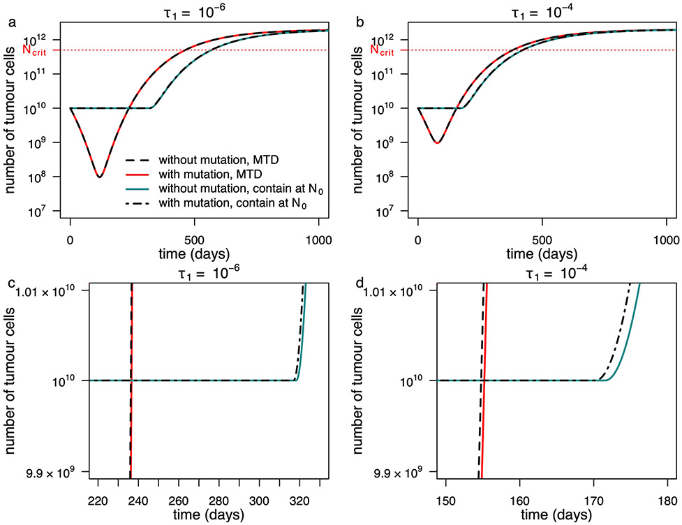
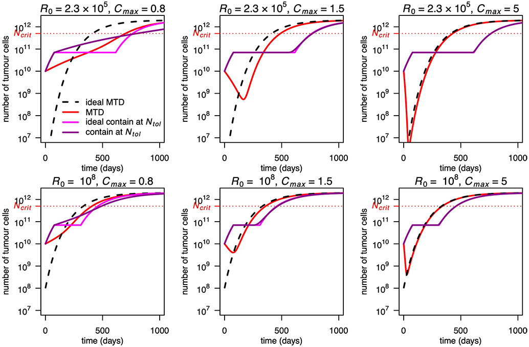
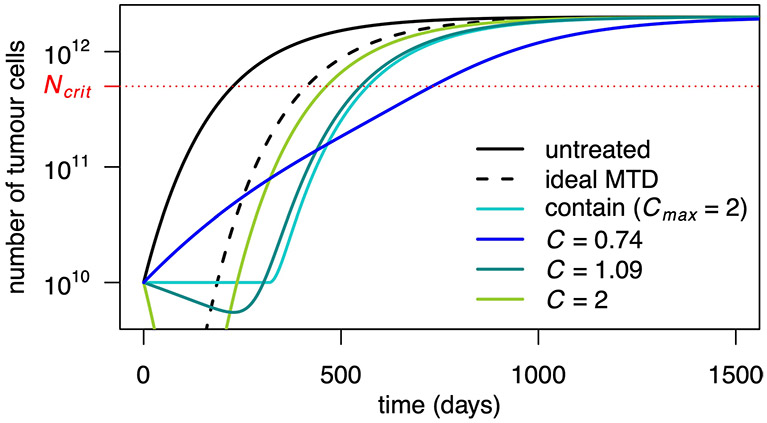
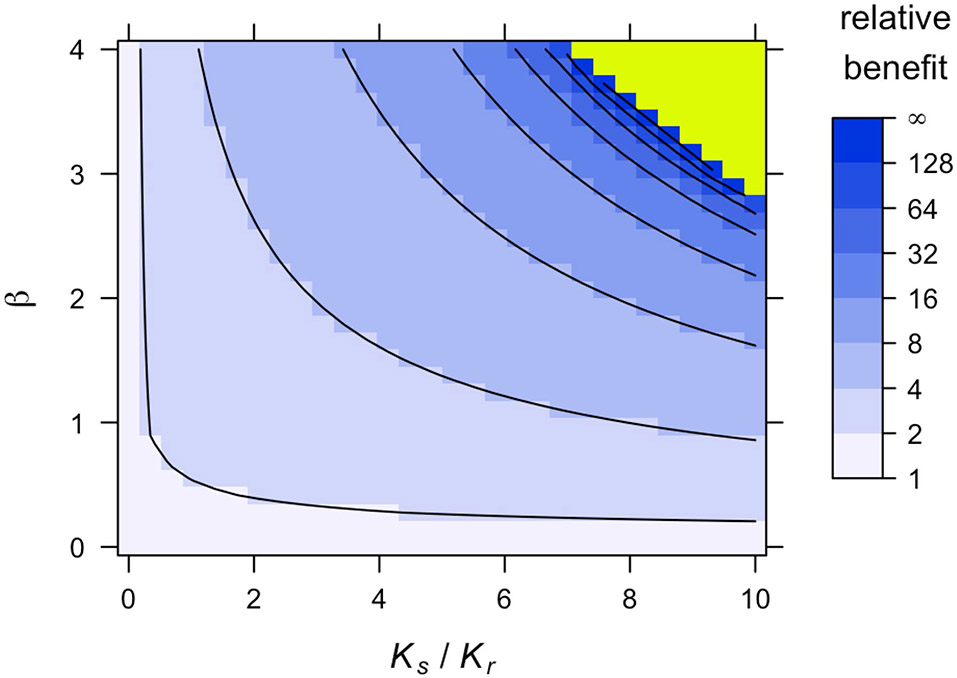
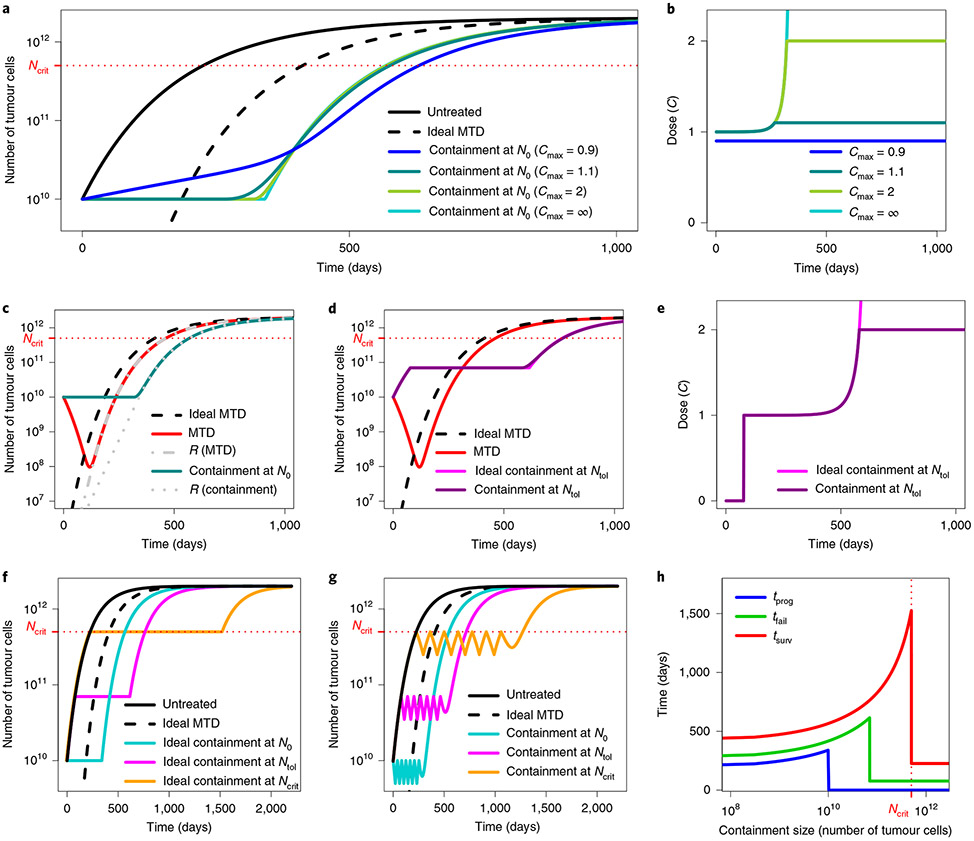
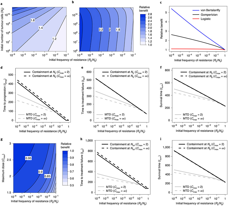
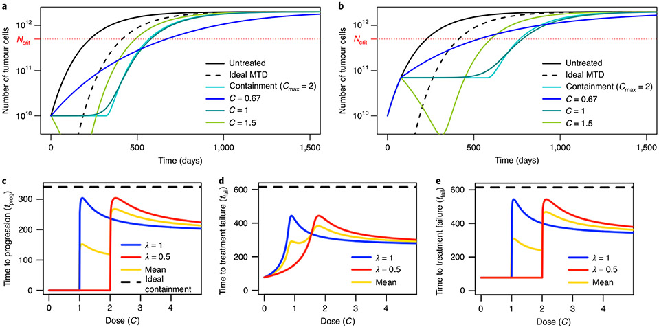
Recent studies have shown that a strategy aiming for containment, not elimination, can control tumour burden more effectively in vitro, in mouse models and in the clinic. These outcomes are consistent with the hypothesis that emergence of resistance to cancer therapy may be prevented or delayed by exploiting competitive ecological interactions between drug-sensitive and drug-resistant tumour cell subpopulations. However, although various mathematical and computational models have been proposed to explain the superiority of particular containment strategies, this evolutionary approach to cancer therapy lacks a rigorous theoretical foundation. Here we combine extensive mathematical analysis and numerical simulations to establish general conditions under which a containment strategy is expected to control tumour burden more effectively than applying the maximum tolerated dose. We show that containment may substantially outperform more aggressive treatment strategies even if resistance incurs no cellular fitness cost. We further provide formulas for predicting the clinical benefits attributable to containment strategies in a wide range of scenarios and compare the outcomes of theoretically optimal treatments with those of more practical protocols. Our results strengthen the rationale for clinical trials of evolutionarily informed cancer therapy, while also clarifying conditions under which containment might fail to outperform standard of care.

Extended Data Fig. 1 ∣. Ideal intermittent containment between N_min and N_max.

Times to progression are shown for ideal intermittent containment between N_min and N₀ for varied N_min value (solid curve), compared to ideal containment at either N₀ (dashed curve) or N_min (dotted curve), according to a Gompertzian growth model (Model 3 in the main text). Non-varied parameter values are as in main text Table 2. The kinks in the curve for ideal intermittent containment are due to the discontinuity of the treatment when a new cycle is completed, or in mathematical terms, to the integer part that appears in the explicit formula.

Extended Data Fig. 2 ∣. Outcomes for five models with different forms of density dependence.

a, Untreated tumour growth curves for a Gompertzian growth model (black curve; Model 3 in the main text), a logistic growth model (red), a von Bertalanffy growth model (blue), an exponential model (yellow) and a superexponential model (grey). Parameter values for the Gompertzian growth model are as in Table 2 of the main text. Parameter values of the logistic and von Bertalanffy models are chosen so that their growth curves are similar to the Gompertzian model for tumour sizes between N₀ and N_crit (the lethal size), as would be the case if the models were fitted to empirical data. In the logistic growth model, K = 6.4×10¹¹ and ρ = 2.4×10⁻². In the von Bertalanffy growth model, K = 5×10¹³, ρ = 90 and γ = 1/3 (the latter value is conventional in tumour growth modelling [24, 37]). In the exponential model, ρ = 0.0175. In the superexponential model, ρ = 4.5×10⁻⁶ and γ = 1/3 (the latter value has been inferred from data [32]). b, Relative benefit, in terms of time to treatment failure, for ideal containment (at size N^tol) versus ideal MTD, for the five models with varied initial frequency of resistance (parameter values are the same as in panel a). Note that relative benefits for all models are independent of ρ.

Extended Data Fig. 3 ∣. Evolution of total tumour size under containment and MTD treatment in a Gompertzian growth model (Model 3 in the main text).

The initial resistant subpopulation size (R₀) is varied. The maximum dose is C_max = 2. Fixed parameter values are as in Table 2 of the main text.

Extended Data Fig. 4 ∣. Containment at N₀ and intermittent containment between N₀ and 0.8 N₀ in a Gompertzian growth model (Model 3 in the main text).

Dashed vertical lines indicate time to progression under containment (dashed grey) and intermittent containment (dashed black). Intermittent containment leads here to a slightly larger time to progression than containment at the upper level. However, as follows from Proposition 6 (Supplementary Material), the resistant population is larger under intermittent containment (red) than under containment (pink). After progression, tumour size quickly becomes larger under intermittent containment (solid black curve) than under containment (solid grey curve). Parameter values are as in Table 2 of the main text.

Extended Data Fig. 5 ∣. Influence of ongoing mutation in a Gompertzian growth model (Model 3 in the main text).

Outcomes are shown for a model in which mutations are neglected after the tumour reaches size N₀ (solid lines) and for a model that explicitly accounts for ongoing mutation from the sensitive to the resistant phenotype at rate τ₁ (broken lines). Two different mutation rates are illustrated. The second row contains the same data as the first row of panels but with different axes so as to make visible the subtle differences between curves. Fixed parameter values are as in Table 2 of the main text.

Extended Data Fig. 6 ∣. Evolution of total tumour size under ideal and non-ideal treatments in a Gompertzian growth model (Model 3 in the main text).

The initial resistant subpopulation size (R₀) and the maximum dose (C_max) are varied. Fixed parameter values are as in Table 2 of the main text.

Extended Data Fig. 7 ∣. Constant dose treatments in a Gompertzian growth model (Model 3 in the main text).

Tumour size for various constant dose treatments are compared to containment at the initial size (subject to C_max = 2), MTD (C = C_max) and ideal MTD. Dose 1.09 maximizes time to progression and 0.74 maximizes survival time among non-delayed constant doses (but is inferior to the optimal delayed constant dose). Parameter values are as in Table 2 of the main text.

Extended Data Fig. 8 ∣. Consequences of costs of resistance in a Gompertzian growth model (Model 4 in the main text).

Relative benefit, in terms of time to treatment failure, for ideal containment (at size N_tol) versus ideal MTD, for varied values of K_r and β. The figure is obtained from simulations, while Fig. 4a in the main text is obtained from our approximate formula. Contour lines are at powers of 2. Fixed parameter values are as in Table 2 of the main text.

Fig. 1 ∣. Illustration of containment and MTD treatments in Model 3.

a, Tumour size under no treatment (black), ideal MTD (dashed) and containment at the initial size for various values of the maximum tolerated dose C_max. The case C_max = ∞ (light blue) corresponds to ideal containment. The patient is assumed to die shortly after tumour size becomes greater than N_crit. b, Drug dose under the containment treatments of a. If C_max < 1, the tumour cannot be stabilized and containment boils down to MTD. c, Tumour size under MTD, ideal MTD and containment at the initial size and resistant population size under MTD and containment. The effect of varying R₀ is illustrated in Extended Data Fig. 3. d, Tumour size under MTD, containment at the maximum tolerable size and their idealized counterparts. The effect of varying C_max is illustrated in Extended Data Fig. 6. e, Drug dose under containment and ideal containment at the maximum tolerable size, as represented in d. f, Tumour size under no treatment, ideal MTD and ideal containment at three different tumour sizes. g, Tumour size under no treatment, ideal MTD and intermittent containment between N_max and N_min = N_max/2 for 3 different values of N_max. h, Times to progression (blue), treatment failure (green) and survival time (red) under ideal containment at a threshold size varied from R₀ to N_crit (ideal containment at R₀ is equivalent to ideal MTD). The time until the tumour exceeds a certain size is maximized by ideal containment at that size. The exact formulas for the idealized treatments are found in the Supplementary Information, section 3.

Fig. 2 ∣. Comparison of clinical benefits of containment and MTD treatments in Model 3.

a, Relative benefit, in terms of time to progression, for ideal containment at size N₀ versus ideal MTD (that is, ratio t_prog(idContN₀)/t_prog(idMTD)), as a function of initial tumour size and frequency of resistant cells. b, Relative benefit, in terms of time to treatment failure, for ideal containment at size N_tol versus ideal MTD (that is, ratio t_fail(idContN_tol)/t_fail(idMTD)), as a function of initial tumour size and frequency of resistant cells. c, Relative benefit, in terms of time to treatment failure, for ideal containment at size N_tol versus ideal MTD for a Gompertzian growth model (black curve; Model 3), a logistic growth model (red) and a von Bertalanffy growth model (blue). Parameter values for the Gompertzian growth model are as in Table 2. Parameter values of the other models are chosen so that untreated tumour growth curves are similar for tumour sizes between N₀ and N_crit (the lethal size). See Extended Data Fig. 2 for details. d–f, Time to progression (d), treatment failure (e) and survival time (f) versus initial frequency of resistance. Outcomes are shown for MTD treatment and containment at N₀, both in the ideal case (C_max = ∞) and subject to C_max = 2. g, Relative benefit, in terms of time to treatment failure for containment versus ideal containment (at size N_tol), as a function of maximum dose threshold (C_max) and initial frequency of resistant cells (the formulas are shown in Supplementary Information, section 3.3). The contour lines are at intervals of 0.05. h,i, Time to treatment failure (h) and survival time (i) versus initial frequency of resistance. Outcomes are shown for MTD treatment and containment at N_tol, both in the ideal case (C_max = ∞) and subject to C_max = 2.

Fig. 3 ∣. Constant dose and delayed constant dose treatments in Model 3.

a, Tumour size for various constant dose treatments compared to containment at the initial size (subject to C_max = 2) and ideal MTD. b, Tumour size for various delayed constant dose treatments (the dose is applied continuously from the first time when N = N_tol) compared to containment at N_tol (subject to C_max = 2) and ideal MTD. Until N = N_tol, all curves are the same, except ideal MTD. c, Times to progression for two patients whose tumours differed in treatment sensitivity (parameter λ) under constant dose treatments, as a function of the dose. The yellow line is the mean of the two patient outcomes and the dashed line is the time to treatment failure under ideal containment at N₀, which is the same for both patients, and the maximal time to progression. d, Times to treatment failure for two patients whose tumours differed in treatment sensitivity under constant dose treatments, as a function of the dose. The yellow line is the mean of the two patient outcomes and the dashed line is the time to treatment failure under ideal containment at N_tol, which is the same for both patients, and the maximal time to treatment failure. e, Times to treatment failure for two patients whose tumours differed in treatment sensitivity under delayed constant dose treatment. (The dose starts to be applied when N = N_tol for the first time.) The yellow line is the mean of the two patient outcomes and the dashed line is the time to treatment failure under ideal containment at N_tol, which was the same for both patients, and the maximal time to treatment failure.

Fig. 4 ∣. Consequences of the costs of resistance in Model 4.

a, Relative benefit, in terms of time to treatment failure, for ideal containment (at size N_tol) versus ideal MTD, for varied values of K_r and β. This figure is based on approximate formulas that are highly accurate for the selected parameter values (Supplementary Information, section 5.2). Extended Data Fig. 8 shows an alternative version of this plot based on simulations. Contour lines are at the power of 2. b, Eventual outcomes of ideal containment (idCont) and ideal MTD (idMTD) treatment strategies based on exact formulas (Supplementary Information, section 5.1). The ‘infinite’ region in a corresponds to the ‘TI’ region in b. Fixed parameter values are as in Table 2.

References

1. Norton L & Simon R Tumor size, sensitivity to therapy, and design of treatment schedules. Cancer Treat. Rep 61, 1307–1317 (1977). - PubMed
1. Goldie JH & Coldman AJ A mathematic model for relating the drug sensitivity of tumors to their spontaneous mutation rate. Cancer Treat. Rep 63, 1727–1733 (1979). - PubMed
1. Gatenby RA A change of strategy in the war on cancer. Nature 459, 508–509 (2009). - PubMed
1. Zhang J, Cunningham JJ, Brown JS & Gatenby RA Integrating evolutionary dynamics into treatment of metastatic castrate-resistant prostate cancer. Nat. Commun 8, 1816 (2017). - PMC - PubMed
1. Martin RB, Fisher ME, Minchin RF & Teo KL Optimal control of tumor size used to maximize survival time when cells are resistant to chemotherapy. Math. Biosci 110, 201–219 (1992). - PubMed
Publication types