. 2021 Jun;24(6):851-862.
doi: 10.1038/s41593-021-00831-7. Epub 2021 Apr 12.

Flexible modulation of sequence generation in the entorhinal-hippocampal system

Affiliations

Flexible modulation of sequence generation in the entorhinal-hippocampal system

Daniel C McNamee et al. Nat Neurosci. 2021 Jun.

Abstract

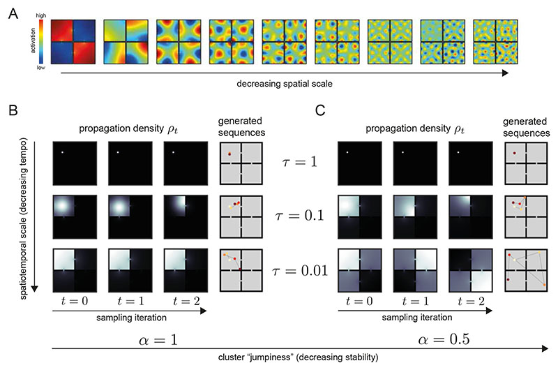
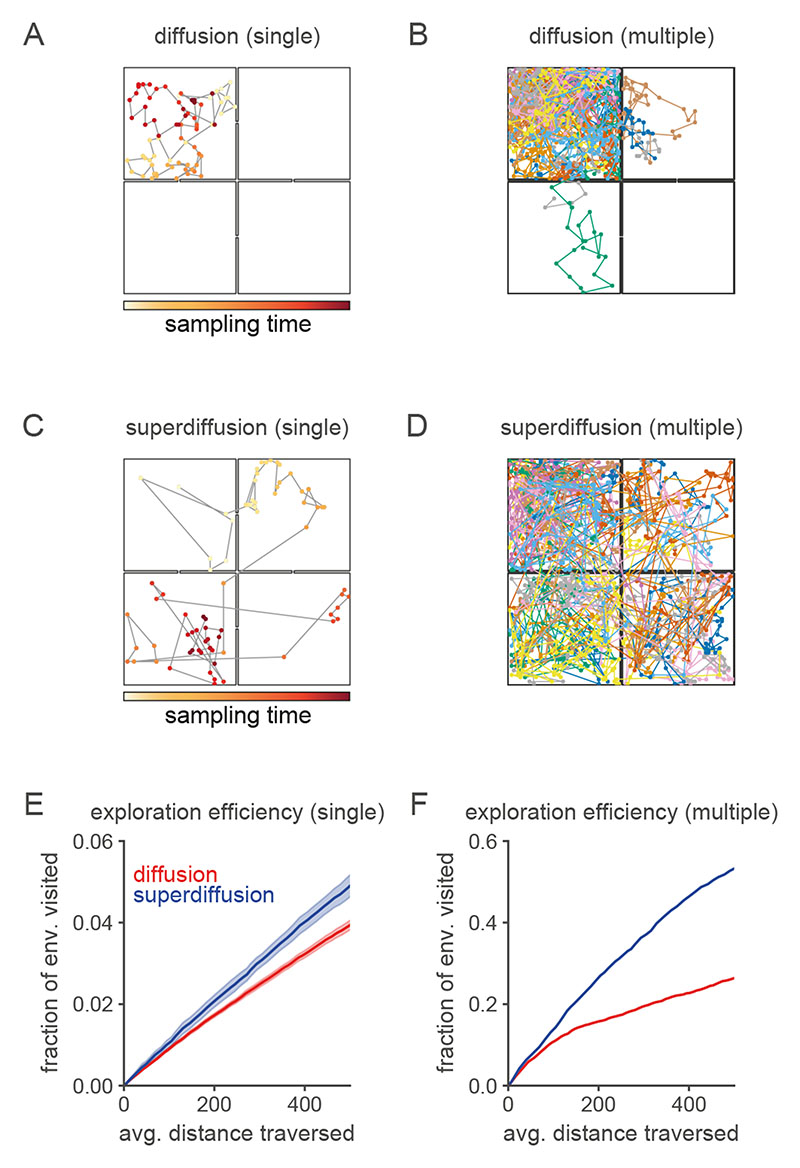
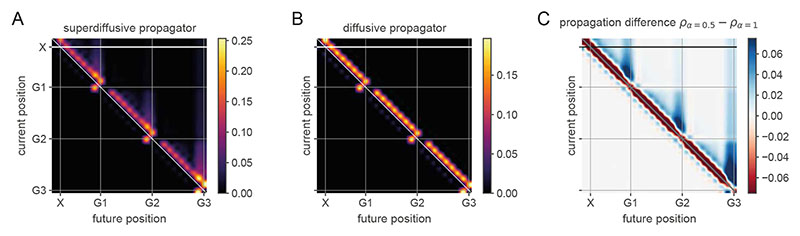
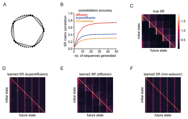
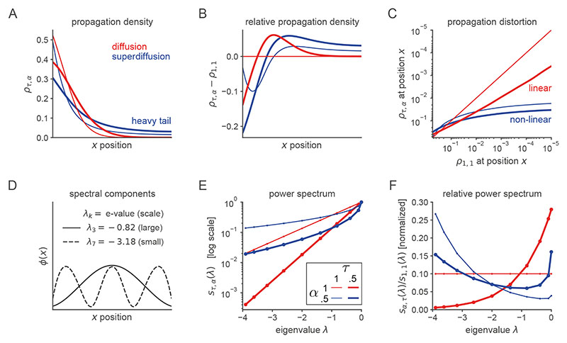
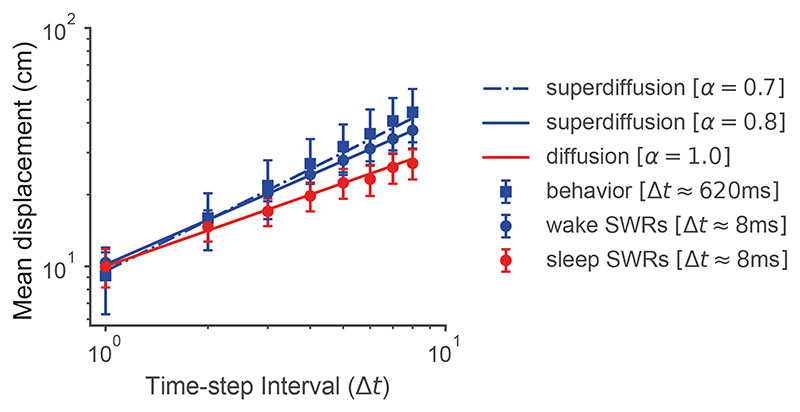
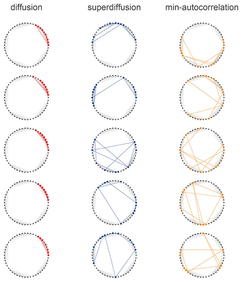
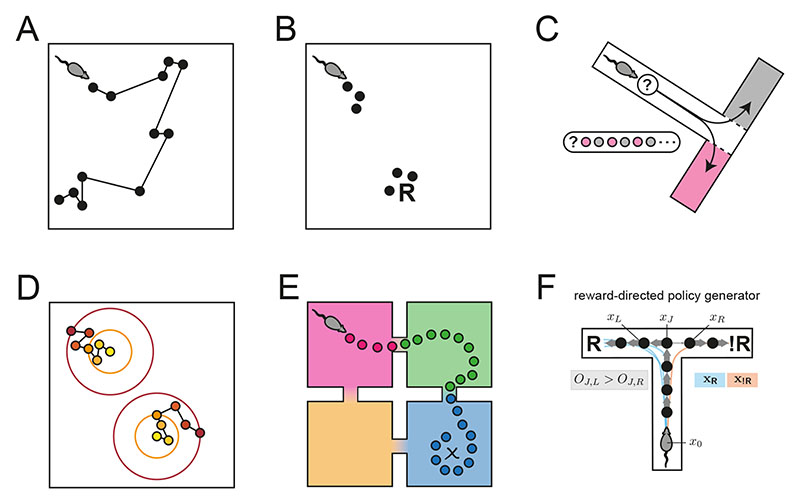
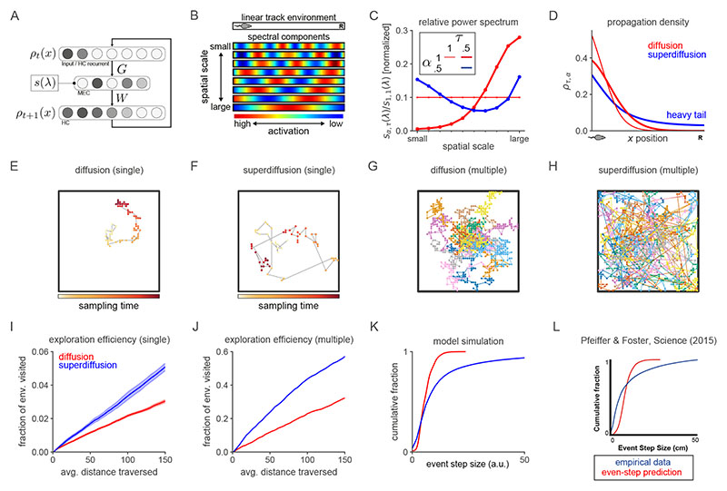
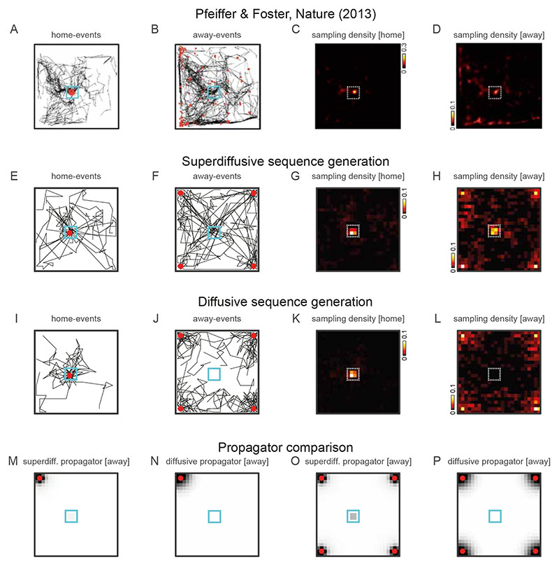
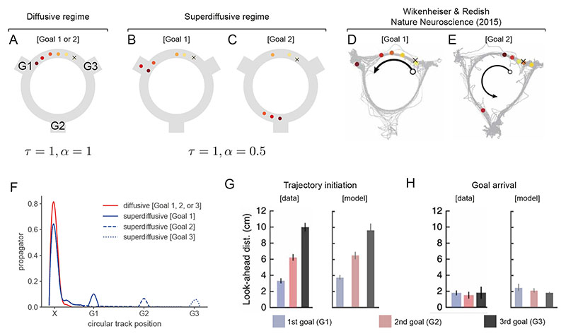
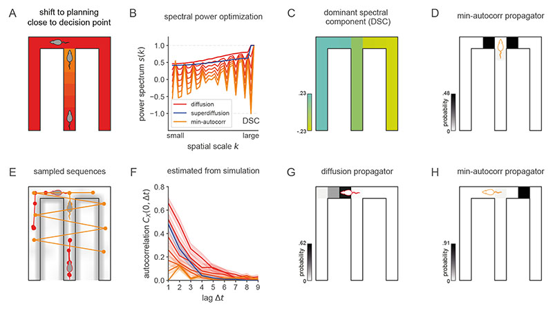
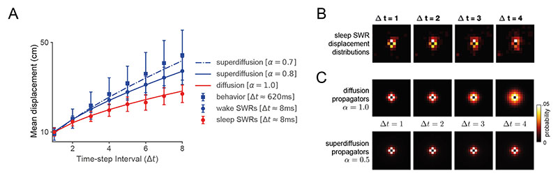
Exploration, consolidation and planning depend on the generation of sequential state representations. However, these algorithms require disparate forms of sampling dynamics for optimal performance. We theorize how the brain should adapt internally generated sequences for particular cognitive functions and propose a neural mechanism by which this may be accomplished within the entorhinal-hippocampal circuit. Specifically, we demonstrate that the systematic modulation along the medial entorhinal cortex dorsoventral axis of grid population input into the hippocampus facilitates a flexible generative process that can interpolate between qualitatively distinct regimes of sequential hippocampal reactivations. By relating the emergent hippocampal activity patterns drawn from our model to empirical data, we explain and reconcile a diversity of recently observed, but apparently unrelated, phenomena such as generative cycling, diffusive hippocampal reactivations and jumping trajectory events.


Conflict of interest statement

Competing Interests

Daniel McNamee and Samuel Gershman declare no competing interests. Kimberly Stachenfeld and Matthew Botvinick are employed by Google DeepMind.

Figures

Figure E1
Figure E1. Sequence generation in an inhomogeneous environment with tempo τ and stability α modulation.
A. Spectral components of the four-room grid world are presented as a function of spatial scale. Generator eigenvectors coincide with the eigenvectors of the corresponding SR. Therefore, many examples of generator eigenvectors may be observed in Ref. [28]. B. As the tempo parameter τ is reduced (with the stability parameter held at α = 1), the power spectrum sτ,α(λ) reweights the spectral components leading to changes in the spatial scale of the propagation densities ρt. C. The generated sequences vary in the extent of their spatiotemporal traversal of the environment.
Figure E2
Figure E2. Exploration efficiency in a structured environment.
The exploration simulation in Fig. 2 is repeated here but for an environment decomposed into four areas connected by bottlenecks. Each area consisted of 50 × 50 states. Simulation parameters were unchanged from Fig. 2 (see Section 5.1.2, Methods). E. Error bands +/- s.e.m. for n = 20 trajectories.
Figure E3
Figure E3. Propagator analysis across all possible current and future positions for the circular track task.
A-B. We plot the superdiffusive (panel A, α = 0.5) and diffusive propagators (panel B, α = 1) for the circular track task for all current positions (y-axis) with all goals activated. The y-axis (x-axis) indexes the current (future) position. Each row reports the probability of each position being sampled given the current position (the row index). C. The difference in diffusive and superdiffusive propagators is plotted. For example, the row corresponding to the initial X position (marked by the thick black line), shows that the local activations are less likely (red) under superdiffusions compared to diffusion (though they are still possible) while remote goal locations specifically are more likely (blue).
Figure E4
Figure E4. Diffusions are optimized for consolidating directed transition structures.
Three regimes of sequence generation are compared in terms of consolidating a directed policy on the same graph used in Fig. 7 where the policy was assumed to be undirected (i.e. a random walk). A. The directed policy is dominated by high probability anti-clockwise transitions (heavy black arrows) between the clique bottleneck states (highlighted by increased size). Within each clique, transitions to the bottleneck state facilitating an anti-clockwise transition to the next clique are relatively likely to occur. B. The same rank order as in Fig. 7C is observed with the diffusive regime leading to the most accurate consolidation of the directed policy successor representation (SR). C. The true directed policy SR. D, E, F. The SRs learned via superdiffusion, diffusion, and minimally autocorrelated sampling respectively. Note that the superdiffusive and minimal autocorrelation regimes identify the the dominant anti-clockwise transition structure but fail to reflect the clustering of states based on their clique membership. This simulation indicates that the diffusive regime is optimal for consolidation regardless of whether the target transition structure corresponds to a random walk or not.
Figure E5
Figure E5. Detailed analyses of spectrally modulated propagation in the linear track environment.
A. Copy of Fig. 2D for context and comparative visualization. B. The propagation distributions in panel A are re-expressed as the difference with respect to the baseline (τ = 1, α =1). C. Each propagation density is plotted against the baseline propagation density (τ = 1, α = 1) on log scales. Note that only superdiffusion results in a non-linear warping of the propagation density. This non-linearity underpins the heavy-tail in the propagation density. D. Small-scale (dashed line) and large-scale (full line) spectral components (i.e., generator eigenvectors) are plotted as a function of linear track position. Eigenvalues take a maximum value of 0 and are ordered according to the spatial scale of the corresponding spectral component. For example, eigenvalues close to zero correspond to large-scale spectral components with the spatial scale of the corresponding spectral component decreasing with the eigenvalue which are always less than or equal to zero. Therefore, the scale of a spectral component ϕk decreases as the absolute value |λk| of its corresponding eigenvalue λk increases. E. Spectral power is plotted as a function of eigenvalue on a log scale. As the tempo τ decreases towards zero, the spatiotemporal horizon increases and the propagation density converges on the stationary state distribution. This corresponds to all spectral components with non-zero eigenvalues decaying to zero. Note that diffusion linearly changes the slope of the power spectrum while superdiffusion imposes a non-linear reweighting. This effect underpins the nonlinear time warping in the propagation densities in panel C. F. The characteristic modulation of the power spectrum under diffusion and superdiffusion is demonstrated by the relative power spectrum sτ,α(λ)s1,1(λ) computed as the power ratio with respect to the baseline propagator. Note that the long-range diffusion propagator (α = 1, τ = 0.5, thick red line) downweights small-scale components and upweights large-scale components while superdiffusion (α = 0.5, τ = 1, thick blue line) relatively upweights both small- and large-scale components but suppresses at medium scales. This enables a superdiffusive propagator to jump to remote positions without traversing intermediate locations.
Figure E6
Figure E6. Mean displacement scales linearly on a log-log plot.
The data and simulations from Fig. 6 are plotted on a logarithmic scales demonstrating the linear relationship between mean spatial displacement and time intervals. Mean displacement (MD) measures the ratio between the spatial displacement and time interval of sequence generation and can be used to infer whether a generative sampling process is operating in a diffusive or superdiffusive regime based on sampled sequences. In particular, the MD function has a slope proportional to α −1 with respect to the time interval Δt (see Section 5.3 Methods). Error bars +/- s.e.m..
Figure E7
Figure E7. Sampled sequences exhibit distinctive patterns across spectral modulation regimes.
Each column shows five sample sequences generated in one of the three sampling regimes studied in Fig. 7. Note that diffusions (left column) tend to remain within a single clique. Superdiffusions (middle column) interleave local diffusions with occasional jumps to other cliques. Jumps are observed as lines crossing the center of the ring which do not conform to any transition step in the underlying state-space structure (grey lines). Minimally autocorrelating propagators (right column) repeatedly generate large jumps between cliques.
Figure 1
Figure 1. In different neurophysiological, behavioral, and cognitive states, distinct modes of sequence generation are active in the entorhinal-hippocampal system.
Drawing on the empirical and computational literatures, we depict several modes of sequence generation supported by our model in a rodent experiment paradigm. Each circle corresponds to a hippocampal place representation, and connecting lines indicate a place activation sequence. A. The exploration patterns of animals and humans, as well as hippocampal place trajectories, interleave large “jumps” between environment positions with local steps consistent with search efficiency optimization. This distinctive regime of sequence generation is referred to as superdiffusive. B. Motivationally salient locations are over-represented in hippocampal activity as reflected in place activations at the reward location (R),. C. Generative cycling refers to the alternating representation of future possibilities in the hippocampal code which occurs during prospective decision-making. Here, the rodent evaluates the candidate behavioral trajectories of turning right (pink) or left (grey) at the junction. D. Diffusive random-walk trajectories are observed in hippocampal reactivations during rest. Colors indicate the successive time steps at which each position is expected to be sampled along each trajectory (from yellow to red). Diffusion implies that, on average, each sampled positions will be spatially displaced from the previous by a similar distance. E. In hierarchical reinforcement learning and human decision-making, environments may be processed across multiple spatiotemporal scales, e.g., using room abstractions in this four-room world. F. In this T-maze task, where a rodent seeks reward R to the left (avoiding the right turn leading to no reward !R), the behavioral policy of the rodent is encoded in the generator O which biases sequence generation to the left xL at the junction xJ. Sequence generation of hypothetical behavioral trajectories xR is then biased towards the reward.
Figure 2
Figure 2. Spectral modulation of grid cell activity alters the statistical structure of hippocampal sequence generation.
A. Abstract entorhinal-hippocampal circuit model. ρt and ρ t+1 are the propagation distributions over environment position at time-steps t and t + 1 respectively. The weight matrices G and W are identified with the generator decomposition O = GΛW. s(λ) is the power spectrum expressed as a function of the generator eigenvalue λ associated with each unit (i.e., spectral component) in the MEC layer. B. Firing maps of units in the MEC layer which exhibit periodic tuning across a range of spatial scales reminiscent of grid cells. Spectral components are equivalently ordered by their eigenvector numbers k and generator eigenvalue magnitudes |λk| from large to small scale. C. Characteristic changes in the power spectrum associated with the diffusive and superdiffusive regimes are highlighted by the corresponding power ratios relative to a baseline. τ-modulated diffusion (α = 1, τ = 0.5, thick red line) results from a downweighting (upweighting) of small-scale (large-scale) spectral components while a-modulated superdiffusion (α = 0.5, τ =1, thick blue line) upweights both small- and large-scale components but suppresses at medium scales. D. Diffusive (α = 1, red lines) versus superdiffusive (α = 0.5, blue line) propagation densities ρτ,α = 1 x0 GSτ,αW in a linear track environment where x 0 corresponds to the location of the rodent. By modulating the tempo τ = 0.5, diffusive propagation can sample over larger distances (thick red line) compared to the baseline diffusion (τ = 1). However, only superdiffusive propagation facilitates an extraordinary jump to the reward (R). Note that these continuous propagation densities have been interpolated from the discrete propagation vectors output by our model. Further technical details are presented in Fig. E5. E-F. Single diffusive (panel E) and superdiffusive (panel F) sequences in an open box environment. The color code from yellow to red reflects the sampling iteration (from the initial sample to the final). Sequences are initialized at the centre of the environment. G-H. Multiple diffusive (panel G) and superdiffusive (panel H) sequences each distinguished by color. I. Mean and standard error of exploration efficiency for individual trajectory simulations (n = 20). J. Parallelized exploration efficiency across all the trajectories in panels G, H. K. Cumulative histogram of step sizes for diffusive trajectories (red) and superdiffusive trajectories (blue). An event refers to the successive representation of two different locations. Step size is measured by Euclidean distance. Therefore the x-axis reflects the Euclidean distance between successively sampled locations during sequence generation. L. Statistical analyses of hippocampal recordings in Ref. [36] indicated that hippocampal trajectory events were superdiffusive since the distribution of step sizes between state activations (blue) was heavy-tailed. This qualitatively matched the simulated cumulative histogram for superdiffusions in panel K in contrast to the prediction (red) based on simulated sequences composed of states separated by equal step sizes. In our model, the latter corresponds to diffusive sequence generation with τ varied to match the velocities exhibited by the recorded trajectory events.
Figure 3
Figure 3. Simulating the over-representation of remote, motivationally salient, locations.
A-D [first row]. Empirical data from Ref. [9]. E-H [second row]. Superdiffusion simulations. I-L [third row]. Diffusion simulations. M-P [fourth row]. Propagators for away events in superdiffusive and diffusive regimes. These are plotted for single location initializations (panels M and N) and for multiple location initializations (panels O and P). A, E, I [first column]. Empirical and simulated trajectory events (black lines) while rodent was located (red circles) at the home location (blue square). B, F, J [second column]. Empirical and simulated trajectory events while rodent was located away from home. C, G, K [third column]. Estimated sampling density for home-events (home location indicated by dotted white square). D, H, L [fourth column]. Estimated sampling density for away-events. This set of panels contains the key comparison. Note that only superdiffusive away-events (panel H) but not diffusive away-events (panel L) remotely over-representation the home location consistent with data (panel D). In our generator model, this is explained by the remote propagation probabilities which are exclusively observed in the superdiffusive regime (panels M and O). Diffusive propagators with sufficiently low tempos (thereby sampling over large spatial scales) can jump from away locations to the home location. The critical distinction is that superdiffusive propagation does not require de-localization to a large spatial scale in order to jump to the home location. Superdiffusions can uncover motivationally salient locations stored locally within the generator regardless of spatial distance.
Figure 4
Figure 4. Theta sequences generated during a goal-directed foraging paradigm exhibited non-local transitions in place coding.
Within individual theta cycles, sequences of place representations in hippocampus emanated from the current position of the rodent (X) and proceeded anti-clockwise around the track with characteristic jumps to one of three goal locations where food was available (labeled G1, G2, G3). Each circle corresponds to a decoded location and the color indicates the temporal order within the sequence (from yellow to red). A. Diffusive sequence generation (a = 1) typically proceeds with localized sequential place activations regardless of the target goal location. B-C. Shifting to the superdiffusive regime (α = 0.5), sequence generation activated local place representations as well as remote goal locations (goal 1 in panel B and goal 2 in panel C) but not intervening locations. D-E. Empirically observed patterns of place activation in theta sequences. Superdiffusive goal-directed sequence generation matches the key qualitative features with goal-directed sequences representing local positions near the animal as well as jumps to goal locations which were over-represented within theta sequences. F. Diffusive propagator and the superdiffusive propagators from the initial X location are plotted. The jumps-to-goals are explained by the unique bumps in the superdiffusive propagators at the remote goal locations. G. The same stability parameter (α = 0.5) generated non-local, goal-jumping trajectories ([model]) with varying look-ahead distances as observed in hippocampal theta sequences ([data], Ref. [11]). Bar heights equal the mean across theta sequences ([data]) or simulated sequences ([model]) and error bars reflect the standard error (n = 50 simulated trajectories). H. Near the goal locations, look-ahead distances were the same across goals since superdiffusive sequence generation is attracted to goals and thus automatically alters the look-ahead distance.
Figure 5
Figure 5. Generative cycling emerges from minimally autocorrelated sequence generation.
A. Spatial alternation task environment from Ref. [12]. We assumed that the well-trained rodent had a decision-making policy composed of moving to the junction, making a binary decision, and then running to the food port at the end of an arm. On approaching the junction where the critical choice is made, we modeled hippocampal sequence generation as shifting from a localized diffusive regime (red) to minimally autocorrelating sampling (orange). B. The minimal autocorrelation (orange), diffusive (red), and superdiffusive (blue) power spectra are plotted. Intermediate colors between red and orange reflect intermediate spectra between purely diffusive and minimally-autocorrelating. Under autocorrelation minimization, we observed that for each positively weighted spectral component, s mac negatively weighted another spectral component of a similar scale. In the EHC, this corresponds to the up- and down-regulation of MEC input into HC in alternation across grid scales. In the generator model, negative spectral modulation drives a generative repulsion depending on the structure of the associated spectral component. The dominant spectral component (DSC) is that which undergoes the largest spectral modulation from diffusion to min-autocorrelation. C. The dominant spectral component reflects a hierarchical decomposition of the state-space into the three arms of the maze. D. At the junction, the minimal autocorrelation propagator splits its propagation density evenly between the two arms in a similar fashion to diffusive propagation. E. While diffusive sequences sweep ahead of the animal in the maze (initialized at the start position and just after a left turn), minimal autocorrelation sequences cycle back and forth between the two arms. F. Estimated autocorrelation CX(0, Δt) as a function of the time interval Δt. Via spectral optimization, the sample autocorrelations were smoothly reduced at all time intervals from pure diffusion to the minimal autocorrelation regime as predicted. Shaded error bands represent SEM (n = 100). G. Just after the turn, the diffusion propagator sweeps ahead of the sampled rodent position. H. Just after the turn, the minimal-autocorrelation propagator switches the sequence generation process to the other arm.
Figure 6
Figure 6. Spatial trajectories encoded in sharp-wave ripples exhibit distinct stability modulation between wake and sleep phases.
A. Blue dots and red dots correspond to the recorded mean displacements (MDs) of spatial trajectories decoded from sharp-wave ripples (SWRs) in the wake phase and sleep phase respectively. There was a difference between the MD slopes (see Section 5.3 Methods) indicating that wake SWRs were generated in the superdiffusive regime (α = 0.8, blue line is the predicted MD curve) while sleep SWRs were diffusive (α = 1, red line is the predicted MD curve). Each of these distinct sampling regimes can be generated by subtly varying the power spectrum sτ α applied to a common underlying environment representation. Note that the physical trajectories of the rodents (“behavior”, blue square markers) were superdiffusive (α = 0.7) consistent with the idea that SWRs may supply candidate exploratory trajectories. This graph is log-log plotted in Fig. E6 where the linearity of mean displacement as a function of time can be observed. Error bars +/- SEM. B. Propagators estimated from reactivated hippocampal trajectories. These resemble those predicted in the diffusive regime but not the superdiffusive regime which lack the increasingly wide spreading activation surrounding the initial position in the center (see panel C). C. Propagators as a function of time interval Δt in the diffusive and superdiffusive regimes.
Figure 7
Figure 7. The performance of cognitive algorithms depends on the sampling regime.
A. We consider a random walk generator on a “ring of cliques” state-space and compare three different sampling regimes (diffusion, superdiffusion, and minimally autocorrelated sampling) with respect to three distinct objectives which quantify the degree to which the sequences generated are optimized for exploration (panel B), learning (panel C), and sampling-based estimation (panel D) respectively. B. Exploration efficiency is defined as the fraction of states explored in an environment relative to the cumulative distance traversed. A steeper slope indicates that more states are explored for less travel distance. With respect to clustered state-spaces (panel A), the characteristic heavy-tail of the superdiffusive propagator implies that occasionally the next state sampled will be drawn from an alternative clique of states unlike diffusion which tends to remain within a single clique (Fig. E7). Minimally autocorrelated sampling is relatively inefficient since it repeatedly samples states across cliques in order to avoid the likelihood of re-sampling nearby states and thus is penalized heavily for traversal distance. C. Consolidation accuracy is the matrix correlation between the learned and true successor representations (SRs). This is plotted as a function of the number of sequences generated. Diffusive replay facilitates the most accurate structure learning of the underlying state-space. D. Sampling coverage is the fraction of states sampled across multiple sequences as a function of the number of sampling iterations. Minimally autocorrelated sampling excels since it is far less likely to resample states within and across sequences. E. The true successor representation matrix for the environment. F-H. The learned successor representations for superdiffusive, diffusive, minimally autocorrelated sequence generation respectively. I-L. Two-dimensional spectral embeddings of the true (panel I) and learned (panels J-L) SRs. The diffusive regime (panel K) successively recapitulates the geometric structure of the true SR (panel I) being composed of five well-spaced cliques of states. In contrast, the SR learned from superdiffusive replay (panel J) does not separate the cliques as clearly due to Lévy jumps leading to the erroneous consolidation of illusory long-range transitions. Minimally autocorrelated sequence generation (panel L) corrupts the spatial structure of the state-space.
Figure 8
Figure 8. Dysregulated spectral modulation cause pathological forms of hippocampal reactivations.
A. An imbalance in the entorhinal power spectrum (purple line) results in turbulent sequence generation. B. As demonstrated in an open box environment, the resulting trajectories essentially sample randomly and thus are inconsistent with the spatiotemporal structure of the environment. C-D. Propagator cross-correlograms organized as a function of place field distance in the diffusion (panel C) and turbulent (panel D) regimes. E. The same analysis of electrophysiological recordings in rodent hippocampus (panel from Ref. [41]) revealed the characteristic V structure as in the structurally-consistent diffusion regime (panel C). Intuitively, the V-structure reflects the fact that it takes time for the process to diffuse over space as a function of the distance between locations. F. In a genetic mouse model of schizophrenia, the time interval between place cell activations in mutant mice did not reflect the spatial distance between the corresponding place fields, and the resulting cross-correlograms resembled those computed in the turbulent regime (panel D).

Similar articles

Cited by

References

    1. Buzsáki G, Moser EI. Memory, navigation and theta rhythm in the hippocampal-entorhinal system. Nature Neuroscience. 2013;16:130–138. - PMC - PubMed
    1. Rowland DC, Roudi Y, Moser MB, Moser EI. Ten Years of Grid Cells. Annual Review of Neuroscience. 2016;39 - PubMed
    1. Lisman J, et al. Viewpoints: how the hippocampus contributes to memory, navigation and cognition. Nature Neuroscience. 2017 - PMC - PubMed
    1. Ólafsdóttir HF, Bush D, Barry C. The Role of Hippocampal Replay in Memory and Planning. Current Biology. 2018;28:R37–R50. - PMC - PubMed
    1. Foster DJ. Replay comes of age. Annual Review of Neuroscience. 2017;40:581–602. - PubMed

Publication types

LinkOut - more resources