Whirligig beetles as corralled active Brownian particles

Abstract

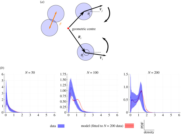
We study the collective dynamics of groups of whirligig beetles Dineutus discolor (Coleoptera: Gyrinidae) swimming freely on the surface of water. We extract individual trajectories for each beetle, including positions and orientations, and use this to discover (i) a density-dependent speed scaling like v ∼ ρ^-ν with ν ≈ 0.4 over two orders of magnitude in density (ii) an inertial delay for velocity alignment of approximately 13 ms and (iii) coexisting high and low-density phases, consistent with motility-induced phase separation (MIPS). We modify a standard active Brownian particle (ABP) model to a corralled ABP (CABP) model that functions in open space by incorporating a density-dependent reorientation of the beetles, towards the cluster. We use our new model to test our hypothesis that an motility-induced phase separation (MIPS) (or a MIPS like effect) can explain the co-occurrence of high- and low-density phases we see in our data. The fitted model then successfully recovers a MIPS-like condensed phase for N = 200 and the absence of such a phase for smaller group sizes N = 50, 100.

Keywords: active Brownian particles; collective motion; inertial delay; insect behaviour; motility-induced phase separation.

Figure 1.

Beetle velocities scale with a power law of local density and exhibit a relatively short inertial delay of 13 ms. (a) A snapshot of the experimental set-up and an overlay detailing the method for local density calculation using the Delaunay tessellation-based method (see methods §4.3). In the overlay, the red points are particle (beetle) positions and lines indicate the Delaunay tessellation. The inset labels the angles and areas used to calculate the local density of the central ith beetle, shown as a red star. The yellow polygon outlined in bold indicates the union of Delaunay triangles having this beetle as a common vertex. We label this set of Delaunay triangles with the index j referring to each triangle as $T_i^{(j)}$, it is area is $A_i^{(j)}$, and the angle subtended at i as ${\theta }_i^{(j)}$. The local density is calculated as the inverse of the average weighted areas $A_i^{(j)}$, with the angles ${\theta }_i^{(j)}$ as weights, further normalized by a factor of 1/2π to account for the fact internal points satisfy $\sum _{\hspace{0.17em}j}{\theta }_i^{(j)}=2\pi$ while points on the boundary satisfy $\sum _{\hspace{0.17em}j}{\theta }_i^{(j)}<2\pi$. See methods section for further details. (b) The relationship between beetle speed v (body lengths per second) and local density ρ (per body length squared) on a log-log scale. Each data point represents a bin-average with error bars showing 1 s.d. The solid black line indicates a power law (ρ^−0.4) as a guide to the eye. (c) Shows the inertial delay between a beetle’s velocity vector and its body axis orientation: the orientation leads the velocity. The shaded ellipses represent the moving outline of the beetle over time. This is quantified in (d), showing the orientation–velocity time correlation function with a Gaussian fit superimposed near the peak, located at Δt = 13 ms (see inset). Only in (d), we use the set of all N = 200 beetle trajectories pre-filtered to remove (near) collisions (see electronic supplementary material for details).

Figure 2.

(a) Cartoon of the model. The particles are treated as soft, self-propelled disks that repel with a force F when overlapped, as in a standard ABP model. However, they also experience a density-dependent re-orientation towards the centre of mass of the swarm (annotated geometric centre), represented by the curved arrows. The reorientation depends on the local density and is assumed strongest at low densities. (b) The density PDFs for the experimental data (blue) and the fitted model (red), evaluated for different numbers of particles N, as shown. The model dynamics correctly recover coexisting dilute and dense phases for N = 200 and a dilute phase alone for N = 50, the phase boundary is around N = 100. The model is parameterized once only, by fitting to the PDF for the N = 200 human tracked dataset; the red curves for N = 50, 100 are the results of this model evaluated with different particle counts. The solid lines are the mean density distributions (kernel density estimates), the error bands indicate 1 s.d. Other simulation parameters in this and subsequent figures are μk = 316.2, D_r = 2.34 rad² s⁻¹ and v₀ = 13.19 body lengths per second.

Figure 3.

Phase diagram for our CABP model in α–τ space, with the one phase (dilute gas) highlighted in red and the two phase (gas and dense liquid) in green. Each of the 14 × 15 sub-panels (the τ = 0 column is excluded) shows the density PDF obtained from a dynamical simulation for N = 200 particles at the corresponding τ, α values (red curve, with s.d. error band). Also shown on each panel is the density PDF from the experimental data at the same N value (blue curve, with s.d. error band, the same on each panel). The best-fit parameters from table 1 correspond roughly to the system shown in row 7, column 9, deep in the two-phase region. The approximate location of the phase boundary denoting the appearance of a high-density phase is identified by eye. Circles overlaid on the plots indicate that we are not confident that the density has reached an equilibrium state for these systems within 30 s real time. This means that the gas phase density may be even smaller than shown; the phase boundary is unaffected. The equilibration time used was between 10 s and 30 s, longer times being required as we move towards the bottom left corner, where re-orientation is weak.

References

1. Fily Y, Marchetti MC. 2012. Athermal phase separation of self-propelled particles with no alignment. Phys. Rev. Lett. 108, 235702. (10.1103/PhysRevLett.108.235702) - DOI - PubMed
1. Palacci J, Sacanna S, Steinberg AP, Pine DJ, Chaikin PM. 2013. Living crystals of light-activated colloidal surfers. Science 339, 936-940. (10.1126/science.1230020) - DOI - PubMed
1. Buttinoni I, Bialké J, Kümmel F, Lüwen H, Bechinger C, Speck T. 2013. Dynamical clustering and phase separation in suspensions of self-propelled colloidal particles. Phys. Rev. Lett. 110, 238301. (10.1103/PhysRevLett.110.238301) - DOI - PubMed
1. Redner GS, Baskaran A, Hagan MF. 2013. Reentrant phase behavior in active colloids with attraction. Phys. Rev. E 88, 012305. (10.1103/PhysRevE.88.012305) - DOI - PubMed
1. Tailleur J, Cates ME. 2008. Statistical mechanics of interacting run-and-tumble bacteria. Phys. Rev. Lett. 100, 218103. (10.1103/PhysRevLett.100.218103) - DOI - PubMed
Publication types