Inferring the function performed by a recurrent neural network

Abstract

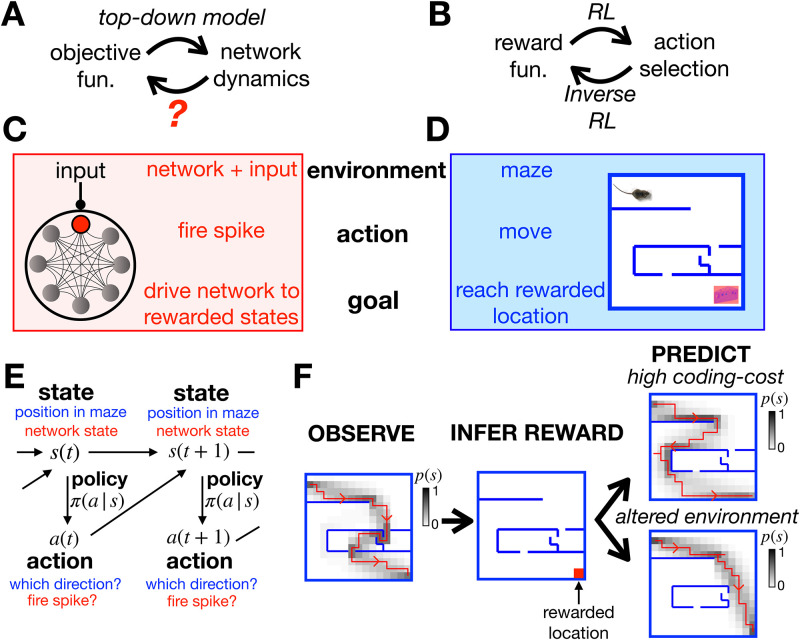
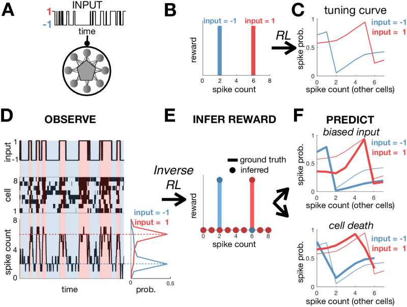
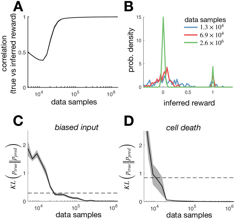
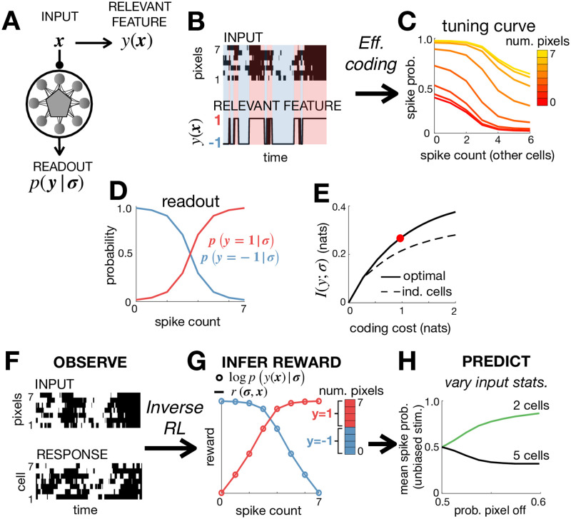
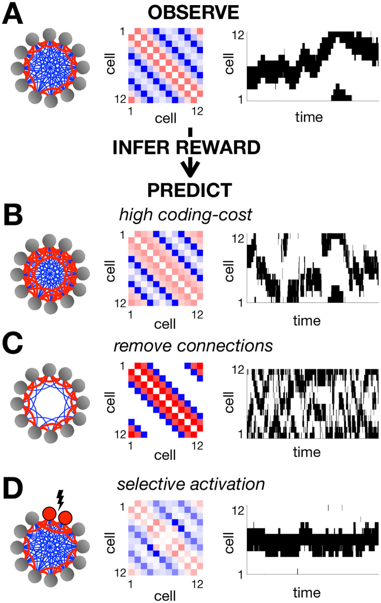
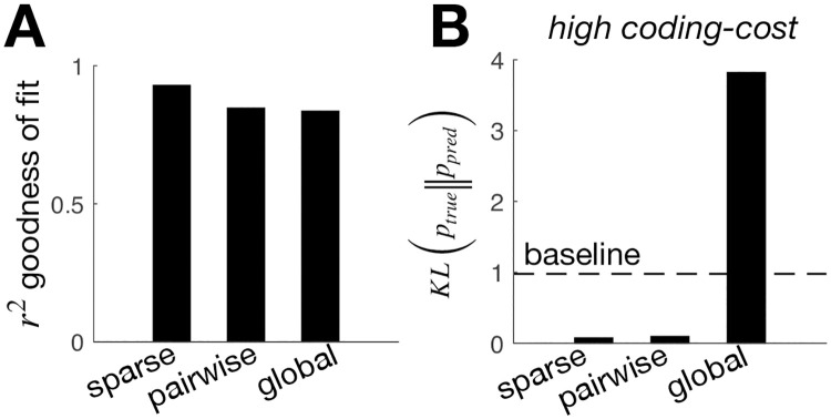
A central goal in systems neuroscience is to understand the functions performed by neural circuits. Previous top-down models addressed this question by comparing the behaviour of an ideal model circuit, optimised to perform a given function, with neural recordings. However, this requires guessing in advance what function is being performed, which may not be possible for many neural systems. To address this, we propose an inverse reinforcement learning (RL) framework for inferring the function performed by a neural network from data. We assume that the responses of each neuron in a network are optimised so as to drive the network towards 'rewarded' states, that are desirable for performing a given function. We then show how one can use inverse RL to infer the reward function optimised by the network from observing its responses. This inferred reward function can be used to predict how the neural network should adapt its dynamics to perform the same function when the external environment or network structure changes. This could lead to theoretical predictions about how neural network dynamics adapt to deal with cell death and/or varying sensory stimulus statistics.

Fig 1. General approach.

(A) Top-down models use an assumed objective function to derive the optimal neural dynamics. The inverse problem is to infer the objective function from observed neural responses. (B) RL uses an assumed reward function to derive an optimal set of actions that an agent should perform in a given environment. Inverse RL infers the reward function from the agent’s actions. (C-D) A mapping between the neural network and textbook RL setup. (E) Both problems can be formulated as MDPs, where an agent (or neuron) can choose which actions, a, to perform to alter their state, s, and increase their reward. (F) Given a reward function and coding cost (which penalises complex policies), we can use entropy-regularised RL to derive the optimal policy (left). Here we plot a single trajectory sampled from the optimal policy (red), as well as how often the agent visits each location (shaded). Conversely, we can use inverse RL to infer the reward function from the agent’s policy (centre). We can then use the inferred reward to predict how the agent’s policy will change when we increase the coding cost to favour simpler (but less rewarded) trajectories (top right), or move the walls of the maze (bottom right).

Fig 2. Training and inferring the function performed by a neural network.

(A) A recurrent neural network receives a binary input, x. (B) The reward function equals 1 if the network fires 2 spikes when x = −1, or 6 spikes when x = 1. (C) After optimisation, neural tuning curves depend on the input, x, and total spike count. (D) Simulated dynamics of the network with 8 neurons (left). The total spike count (below) is tightly peaked around the rewarded values. (E) Using inverse RL on the observed network dynamics, we infer the original reward function used to optimise the network from its observed dynamics. (F) The inferred reward function is used to predict how neural tuning curves will adapt depending on contextual changes, such as varying the input statistics (e.g. decreasing p(x = 1)) (top right), or cell death (bottom right). Thick/thin lines show adapted/original tuning curves, respectively.

Fig 3. Inferring the reward from limited data.

(A) The r²-goodness of fit between the true reward, and the reward inferred using a finite number of samples (a sample is defined as an observation of the network state at a single time-point). The solid line indicates the r² value averaged over 20 different simulations, while the shaded areas indicate the standard error on the mean. (B) Distribution of rewards inferred from a variable numbers of data samples. As the number of data samples is increased, the distribution of inferred rewards becomes more sharply peaked around 0 and 1 (reflecting the fact that the true reward was binary). (C) The KL-divergence between the optimal response distribution with altered input statistics (see Fig 2F, upper) and the response distribution predicted using the reward inferred in the initial condition from a variable number of samples. The solid line indicates the KL-divergence averaged over 20 different simulations, while the shaded areas indicate the standard error on the mean. A horizontal dashed line indicates the KL-divergence between the response distribution with biased input and the original condition (that was used to infer the reward). (D) Same as panel (C), but where instead of altering the input statistics, we remove cells from the network (see Fig 2F, lower).

Fig 4. Efficient coding and inverse RL.

(A) The neural code was optimised to efficiently encode an external input, x, so as to maximise information about a relevant stimulus feature y(x). (B) The input, x consisted of 7 binary pixels. The relevant feature, y(x), was equal to 1 if >3 pixels were active, and -1 otherwise. (C) Optimising a network of 7 neurons to efficiently encode y(x) resulted in all neurons having identical tuning curves, which depended on the number of active pixels and total spike count. (D) The posterior probability that y = 1 varied monotonically with the spike count. (E) The optimised network encoded significantly more information about y(x) than a network of independent neurons with matching stimulus-dependent spiking probabilities, p(σ_i = 1|x). The coding cost used for the simulations in the other panels is indicated by a red circle. (F-G) We use the observed responses of the network (F) to infer the reward function optimised by the network, r(σ, x) (G). If the network efficiently encodes a relevant feature, y(x), then the inferred reward (solid lines) should be proportional to the log-posterior, logp(y(x)|σ) (empty circles). This allows us to (i) recover y(x) from observed neural responses, (ii) test whether this feature is encoded efficiently by the network. (H) We can use the inferred objective to predict how varying the input statistics, by reducing the probability that pixels are active, causes the population to split into two cell types, with different tuning curves and mean firing rates (right).

Fig 5. Pairwise coupled network.

(A) We optimized the parameters of a pairwise coupled network, using a reward function that was equal to 1 when exactly 4 adjacent neurons were simultaneously active, and 0 otherwise. The resulting couplings between neurons are schematized on the left, with positive couplings in red and negative couplings in blue. The exact coupling strengths are plotted in the centre. On the right we show an example of the network dynamics. Using inverse RL, we can infer the original reward function used to optimise the network from its observed dynamics. We can then use this inferred reward to predict how the network dynamics will vary when we increase the coding cost (B), remove connections between distant neurons (C) or selectively activate certain neurons (D).

Fig 6. Effect of assuming different types of reward function.

We compared the inferred reward when we assumed a sparse model (i.e. a small number of states associated with non-zero positive reward) a pairwise model (i.e. the reward depends on the first and second-order response statistics) and a global model (i.e. the reward depends on the total number of active neurons only). (A) r² goodness of fit between the true and the inferred reward, assuming a sparse, pairwise, or global model. (B) The KL-divergence between the optimal response distribution with high coding cost (see Fig 5B) and the response distribution predicted using the reward inferred in the initial condition, assuming a sparse, pairwise, or global model. A horizontal dashed line indicates the KL-divergence between the response distribution with high coding cost and the original condition (that was used to infer the reward).

References

1. Yang GR, Joglekar MR, Song HF, Newsome WT, Wang XJ. (2019). Task representations in neural networks trained to perform many cognitive tasks. Nat Neurosci, 22: 297–306 10.1038/s41593-018-0310-2 - DOI - PMC - PubMed
1. Heeger DJ (2017) Theory of cortical function. Proc Natl Acad Sci USA 114: 1773–1782 10.1073/pnas.1619788114 - DOI - PMC - PubMed
1. Sussillo D, Abbott LF (2009) Generating coherent patterns of activity from chaotic neural networks. Neuron 63: 544–557. 10.1016/j.neuron.2009.07.018 - DOI - PMC - PubMed
1. Gütig R (2016) Spiking neurons can discover predictive features by aggregate–label learning. Science 351(6277): aab4113 10.1126/science.aab4113 - DOI - PubMed
1. Hopfield JJ (1982) Neural networks and physical systems with emergent collective computational abilities. Proc Natl Acad Sci USA 79: 2554–2558 10.1073/pnas.79.8.2554 - DOI - PMC - PubMed
Publication types
LinkOut - more resources