Neuropixels 2.0: A miniaturized high-density probe for stable, long-term brain recordings

Abstract

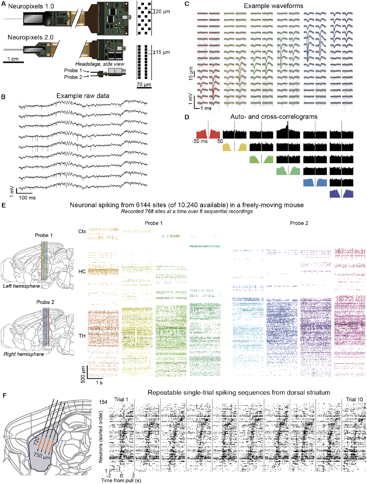
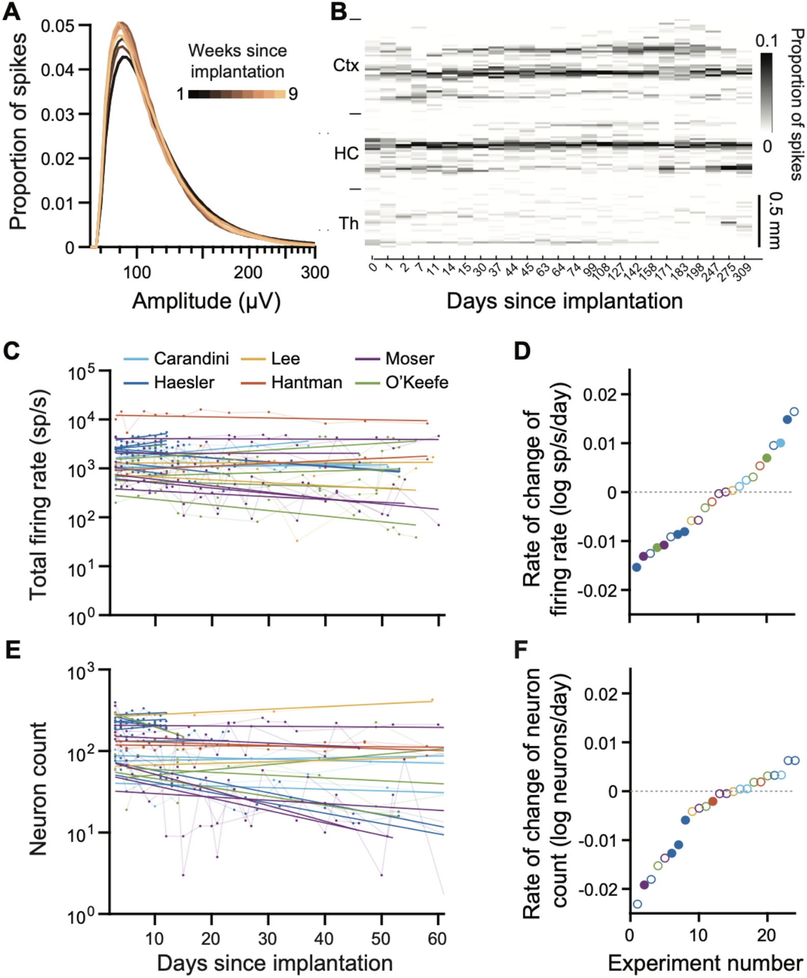
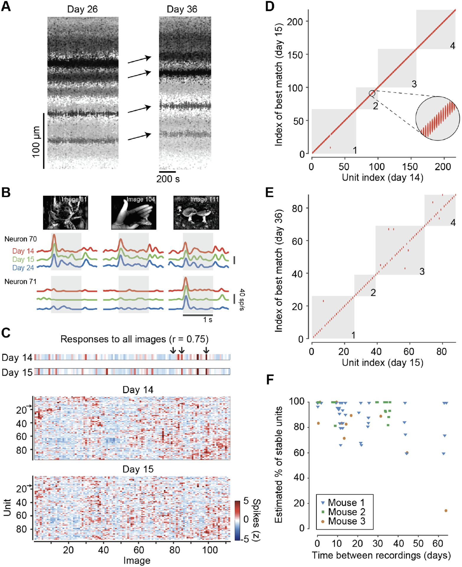
Measuring the dynamics of neural processing across time scales requires following the spiking of thousands of individual neurons over milliseconds and months. To address this need, we introduce the Neuropixels 2.0 probe together with newly designed analysis algorithms. The probe has more than 5000 sites and is miniaturized to facilitate chronic implants in small mammals and recording during unrestrained behavior. High-quality recordings over long time scales were reliably obtained in mice and rats in six laboratories. Improved site density and arrangement combined with newly created data processing methods enable automatic post hoc correction for brain movements, allowing recording from the same neurons for more than 2 months. These probes and algorithms enable stable recordings from thousands of sites during free behavior, even in small animals such as mice.

Figure 1.. Neuropixels 2.0 probes are miniaturized and provide high-quality recordings across thousands of sites in vivo.

(A) Comparison of the NP 1.0 (top) and 2.0 (bottom) devices. NP 2.0 have four shanks (or a single shank, not shown), miniaturized rigid base and headstage, and increased recording site density (right). They allow for two probes to be attached to a single headstage (inset). (B) Example raw data traces show local field potentials and spiking signals recorded from 9 nearby recording sites in the olfactory bulb in an awake, head-fixed mouse. (C) Example spike waveforms from six selected neurons recorded on overlapping channels. The mean waveform (color) is overlaid on 50 randomly selected individual waveforms (grey). (D) Auto- and cross-correlograms (colored and black plots, respectively) of the example neurons from panel C, shown over a −50 to +50 ms window. (E) Example spiking rasters from two NP 2.0 probes chronically implanted in a single mouse, showing spikes recorded on 6,144 sites, out of the 10,240 sites available across the two probes. Each colored block represents spike times recorded from a ‘bank’ of 384 channels and plotted at the depth along the probe at which they occurred. Each probe could record one bank at a time, so that two banks (768 sites), were recorded simultaneously. The 6,144 sites were accessed by altering switches in software, and recording over 8 sequential recording epochs of 768 sites. (F) Dense local recordings from dorsal striatum in head-fixed mice performing a joystick-pulling task reveal reliable sequences of spiking activity on individual trials. Left, the 384 simultaneously recorded sites (orange) cover a plane 720 × 750 μm in extent, covering a significant proportion of dorsal striatum (purple). Recording location is illustrative, and does not represent a reconstruction from histology. Right, spiking raster from ten trials reveals characteristic spiking sequences across neurons. The neurons were sorted for latency of average peak response and are shown in the same order on each trial.

Figure 2.. Chronic recordings with Neuropixels 2.0 probes maintained high yield for >8 weeks.

(A) Stable distribution of spike amplitudes recorded across weeks (averages of n=14 subjects). Spike amplitude distributions from recordings made on each week are superimposed and color-coded by weeks since implantation. (B) Firing rates across channels are stable over nearly a year, in cortex (Ctx), hippocampus (HC), and thalamus (TH) in an example recording. Spikes are spatially binned across 15 μm. The spike counts at each depth are normalized by the total spike count within a recording day, so that the color scale reflects the proportion of spikes found at each depth on a given day. (C) Total firing rates over the course of 60 days for all probes used in this study. A linear regression line (in log₁₀ units) was fitted to the total firing rate of each probe versus days since implantation. The color of each series represents data collected in different laboratories. Note that different brain regions were targeted by each lab and each implant, likely accounting for much of the variability across implants. Nevertheless, total firing rates are unchanging or changing slowly for all tested recording targets. (D) Rate of change in log total firing rate extracted from the linear fits (slope) of each experiment in C. Each point represents one experiment. A rate of −0.01 log units per day indicates that over 100 days, the value declines by one log unit, i.e. a factor of 10. Filled dots represent significant correlations of the firing rate (or cluster count) with time. (E) Rate of change in log yield of spike-sorted neurons for each probe over the course of 60 days. (F) Same as D for neuron yields.

Figure 3.. Post-hoc computational motion correction yields stable recordings even in the face of electrode motion.

(A) Typical brain movements are parallel to the probe shank (blue arrows); they were simulated by moving the probe up and down along the same axis while recording (red arrows). (B) Movements of the brain relative to a stationary probe. A spiking raster with spikes plotted at the position they occurred along the probe. Darker spikes have larger amplitude. The shared movement of the traces across depth reveals relative motion of neurons across the whole probe over both fast (<1 min) and slow (~10 min) timescales. (C) The motion correction algorithm counts spikes by depth and amplitude in 2 s time bins to create ‘images’ of neural activity that are registered across time. (D) The estimated position over time (colored traces) for an example recording made with imposed probe motion (black). Each color represents the position estimated at a different depth along the probe (see Fig. S5). (E) Raw data segments showing the motion correction approach. Left: a raw data segment from 14 channels where position was estimated near zero relative to the recording’s zero point. Middle: raw data from a later time point where position was estimated to be 53.0 μm from the zero point (a shift of ~3.5 sites). Right: the results of correcting those raw data (through resampling and spatial interpolation) to shift it to position = 0. All spikes are shifted downward by this process, and the large spike to the left now aligns with the large spike from the first sample, presumably from the same neuron. (F) Spiking raster of a segment of an example recording with spikes plotted at the depth they occurred on the probe. The triangle-wave pattern of imposed probe motion (red) is reflected in the movement of spikes along the probe during the middle of the recording. Blue dashed box: the segment of data enlarged in panel B, to illustrate naturally occurring brain motion. (G) Raster of spikes detected after applying the motion correction algorithm, showing correction of both imposed motion and naturally occurring motion. (H) The motion correction algorithm improved stability measured as the absolute value of the correlation coefficient between firing rates and probe-brain motion. (I) The motion correction algorithm improved yield of neurons whose firing rates had no correlation with the imposed motion (“stable”) and reduced the number whose firing rates correlated with the motion (“unstable”).

Figure 4.. Neuropixels 2.0 probes with motion correction allow successful recording of hundreds of neurons across days and weeks.

(A) Data from an example mouse with a chronic NP 2.0 probe in visual cortex, showing significant drift between recordings on consecutive days. Plotting conventions as in Fig 3b. (B) Firing rate of an example neuron in response to three images presented for 1 s (gray box), averaged over n=5 repetitions, on each of three days (red, green, blue) (C) Top: Average spike count response (z-scored) of the same neuron to all the images in the battery (arrows indicate the 3 example images from b. The responses have a correlation of 0.75 across the two days. Bottom: Example average spike count response of all units with visual fingerprint on one of the shanks on two consecutive recording days, with both neurons and images in sorted order according to similarity of responses. Color bar: z-scored response. (D) To gauge unit stability, each unit’s visual fingerprint on the first day was matched with its own fingerprint and with the fingerprint of the physically closest other unit (not necessarily labeled with a consecutive index) on the second day. All units matched to themselves (points on the diagonal, 216/217), except for one that matched better with the visual fingerprint of its neighbor (single red point off the diagonal in shank 1). Gray squares separate the four shanks (numbered). (E) Same format as D, for two recordings made three weeks apart (79/88 units are matches). (F) Summary of stability of well-isolated units across 26 spliced pairs of recordings in three mice. Each point represents a single shank, and data from each mouse is shown by a different symbol. In total, 1,748 well-isolated units with visual fingerprints were analyzed. The estimated percentage of stable units is calculated as 2Pr(match) – 1 where Pr(match) is the probability that a unit’s visual fingerprint matched more closely than the nearest neighbor on the two days (see Methods for derivation). For presentation purposes only, points were jittered along the x-axis to avoid overlaps. Note that the interval between implantation and the first recording in each pair of recordings was variable, in some cases exceeding 6 months.

Figure 5.. Neuropixels 2.0 probes allow recording from twice as many sites as the number of recording channels.

(A) Sites from multiple banks connect to a single set of recording channels, showing 10 sites out of 384 for each bank. Software controls allow switching the channels to the sites in bank 1 (left), in bank 2 (middle) or in both banks concurrently (right). To allow unmixing, the mapping from bank 2 sites to channels is scrambled relative to bank 1. (B) Spiking raster (conventions as in Fig 3b) from recordings with all three configurations. When bank 1 and bank 2 are recorded together (right), spikes are plotted at their inferred locations based on the mismatch score of their source template. As expected, in this condition the spike amplitudes are lower by a factor of two.

References

1. Chen R, Canales A, Anikeeva P, Neural recording and modulation technologies. Nat. Rev. Mater 2, 1–16 (2017). - PMC - PubMed
1. Seymour JP, Wu F, Wise KD, Yoon E, State-of-the-art MEMS and microsystem tools for brain research. Microsyst. Nanoeng 3, 1–16 (2017). - PMC - PubMed
1. Steinmetz NA, Koch C, Harris KD, Carandini M, Challenges and opportunities for large-scale electrophysiology with Neuropixels probes. Curr. Opin. Neurobiol 50, 92–100 (2018). - PMC - PubMed
1. Hong G, Lieber CM, Novel electrode technologies for neural recordings. Nat. Rev. Neurosci 20, 330–345 (2019). - PMC - PubMed
1. Kleinfeld D, Luan L, Mitra PP, Robinson JT, Sarpeshkar R, Shepard K, Xie C, Harris TD, Can One Concurrently Record Electrical Spikes from Every Neuron in a Mammalian Brain? Neuron. 103, 1005–1015 (2019). - PMC - PubMed
Publication types