Democratising deep learning for microscopy with ZeroCostDL4Mic

Abstract

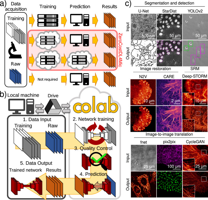
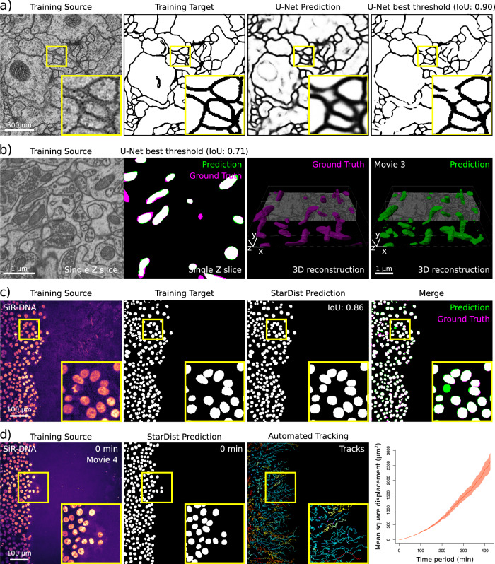
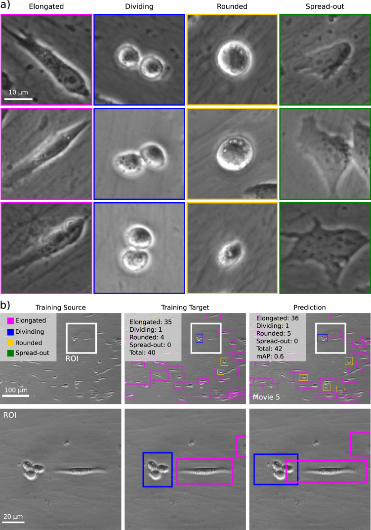
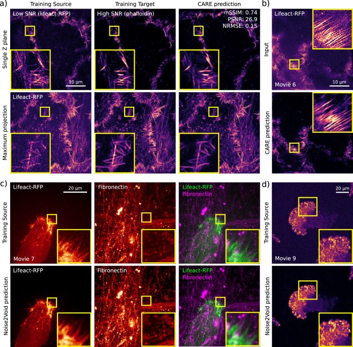
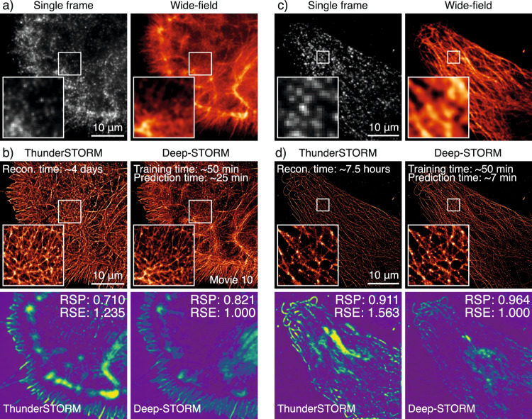
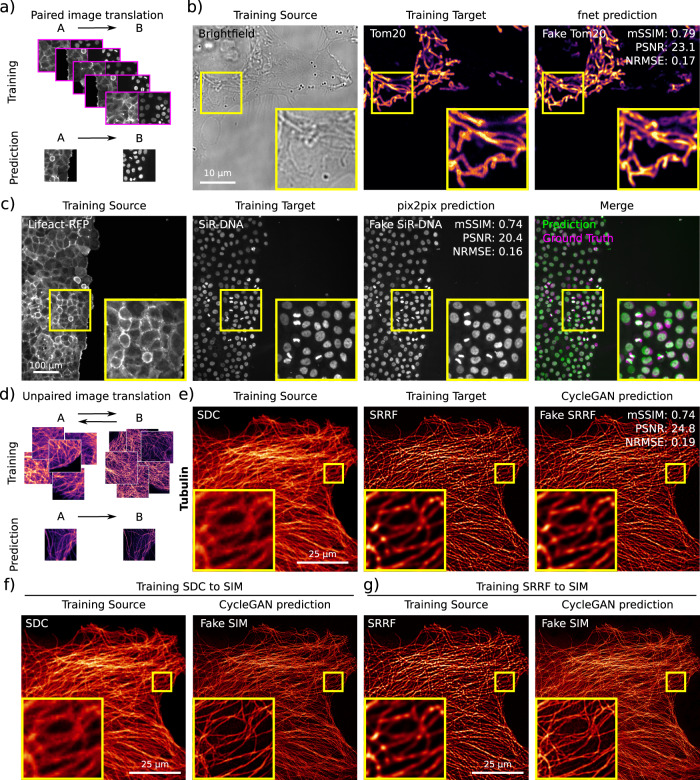
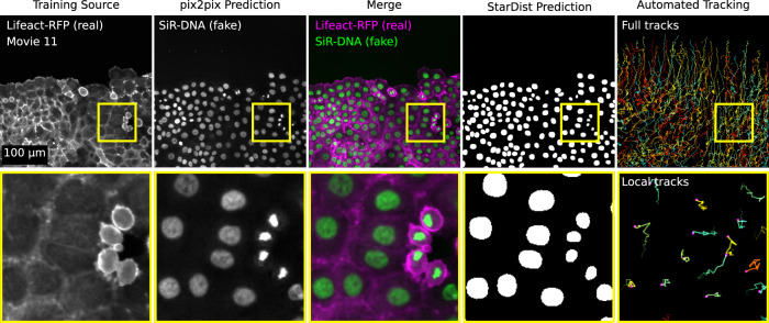
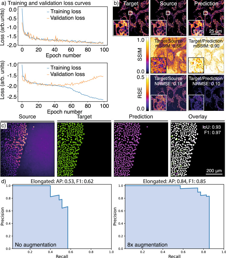
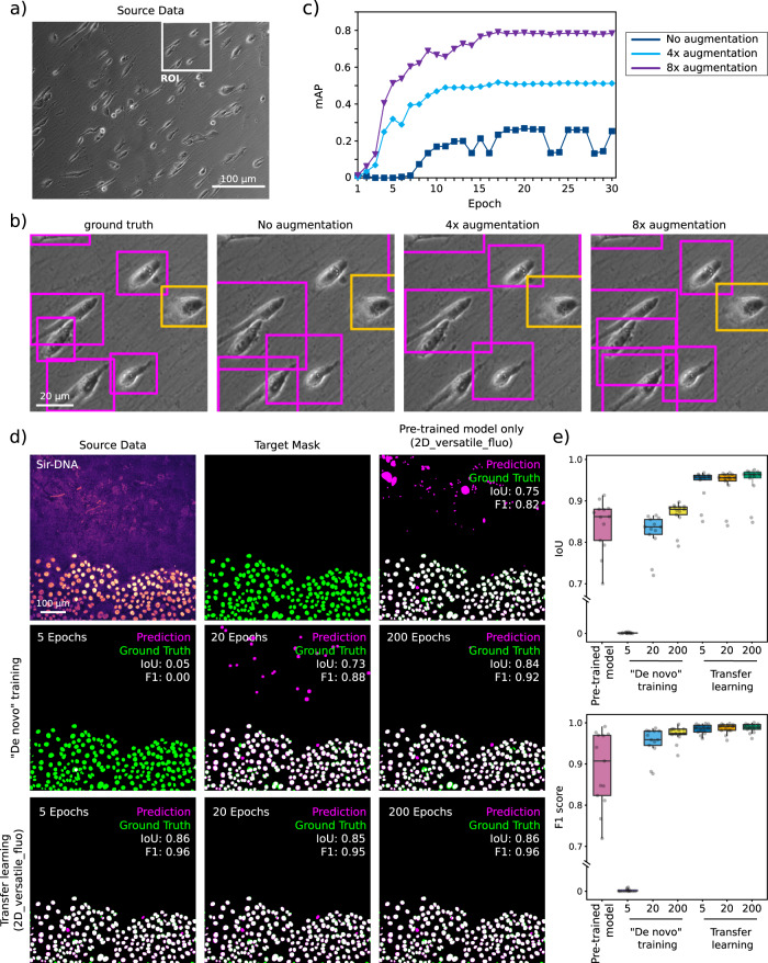
Deep Learning (DL) methods are powerful analytical tools for microscopy and can outperform conventional image processing pipelines. Despite the enthusiasm and innovations fuelled by DL technology, the need to access powerful and compatible resources to train DL networks leads to an accessibility barrier that novice users often find difficult to overcome. Here, we present ZeroCostDL4Mic, an entry-level platform simplifying DL access by leveraging the free, cloud-based computational resources of Google Colab. ZeroCostDL4Mic allows researchers with no coding expertise to train and apply key DL networks to perform tasks including segmentation (using U-Net and StarDist), object detection (using YOLOv2), denoising (using CARE and Noise2Void), super-resolution microscopy (using Deep-STORM), and image-to-image translation (using Label-free prediction - fnet, pix2pix and CycleGAN). Importantly, we provide suitable quantitative tools for each network to evaluate model performance, allowing model optimisation. We demonstrate the application of the platform to study multiple biological processes.

Fig. 1. Using DL for microscopy.

a Paths to exploiting DL. Training on local servers and inference on local machines (or servers) (first row), cloud-based training and local inference (second row), cloud-based training and inference (third row) and pretrained networks on standard machines (fourth row). b Overview of ZeroCostDL4Mic. The workflow of ZeroCostDL4Mic, featuring data transfer through Google Drive, training, quality control and prediction via Google Colab. After running a network, trained models, quality control and prediction results can then be downloaded to the user’s machine. c Overview of the bioimage analysis tasks currently implemented within the ZeroCostDL4Mic platform. Datasets from top left to bottom right: U-Net—ISBI 2012 Neuronal Segmentation Dataset^,, StarDist—nuclear marker (SiR-DNA) in DCIS.COM cells, YOLOv2—bright field in MDA-MB-231 cells, N2V—actin label (paxillin-GFP) in U-251-glioma cells, CARE—actin label Lifeact-RFP in DCIS.COM cells, Deep-STORM—actin-labelled glial cell, fnet—bright-field and mitochondrial label TOM20-Alexa Fluor 594 in HeLa cells, pix2pix—actin label Lifeact-RFP and nuclear labels in DCIS.COM cells, CycleGAN—tubulin label in U2OS cells. All datasets are available through Zenodo (see “Data availability”) or as indicated in the GitHub repository.

Fig. 2. Image-segmentation networks (U-Net and StarDist).

a, b Example of data generated using the ZeroCostDL4Mic U-Net and StarDist notebooks. a A 2D U-Net model was trained to segment neuronal membranes from EM images. This training dataset is from the 2012 ISBI segmentation challenge. Training source (raw data), training targets (hand-annotated binary masks), predictions (raw output of the notebook after training) and U-Net image thresholded output are displayed, achieving an Intersection over Union (IoU) of 0.90 (see Supplementary Note 2 for details). The optimal threshold was assessed automatically using the Quality Control section of the notebook (see Supplementary Note 3). b A 3D U-Net network was trained to segment mitochondria from EM images. The training dataset was made available by EPFL and consists of EM images of 5 × 5 × 5 µm³ sections taken from the CA1 hippocampus region of the brain. A representative single Z slice, as well as an overlay displaying U-Net prediction and the ground truth, are displayed. 3D reconstructions displayed were performed from U-Net predictions using Imaris (Supplementary Movie 3). c, d Example of data generated using the ZeroCostDL4Mic StarDist notebooks. c, d A StarDist model was trained (c) to automatically detect nuclei in movies of migrating DCIS.COM cells, labelled with SiR-DNA, to track their movement automatically (d). c Example of Training source (DCIS.COM cells labelled with SiR-DNA), Training targets (Ground-truth masks) and StarDist prediction (IoU of 0.86) are displayed. d StarDist outputs were used to automatically track cell movement over time in TrackMate (Supplementary Movie 4). Cell tracks were further analysed using the online platform motilitylab.net, indicating a directed movement that is expected for such migration assays (error bars represent the standard deviation). IoU Intersection over Union.

Fig. 3. Object detection (YOLOv2).

Example of data generated using the ZeroCostDL4Mic YOLOv2 notebook, detecting and identifying cell shape classification from a cell migration bright-field time-lapse dataset. a Identified cell shapes and representative examples that were hand-labelled in the training dataset. b Input, ground truth and prediction obtained from object detection, highlighting the identification of the presence of three classes in the field-of-view (see also Supplementary Movie 5) and an mAP of 0.60 for this field of view. mAP: mean average precision (see Supplementary Note 2 for details). mAP mean average precision.

Fig. 4. Image denoising and restoration networks (CARE and Noise2Void).

Example of data generated using ZeroCostDL4Mic CARE and Noise2Void notebooks. a, b A 3D CARE network was trained using SIM images of the actin cytoskeleton of DCIS.COM cells using fixed samples (a) to denoise live-cell imaging data (b). Quality control metrics are as follows: mSSIM: 0.74, PSNR: 26.9 and NRMSE: 0.15. c Fixed samples were imaged using SIM to obtain low signal-to-noise images (lifeact-RFP, Training Source) and matching high signal-to-noise (Phalloidin staining, Training Target) images, and this paired dataset was used to train CARE. Input, ground truth and a CARE prediction are displayed (both single Z plane and maximal projections). The QC metrics values computed directly in the CARE notebook are indicated. b The network trained in (a) was then used to restore live-cell imaging data (Supplementary Movie 6). The low SNR image (input) and the associated CARE predictions are displayed (single plane). c Movie of an ovarian carcinoma cell labelled with lifeact-RFP migrating on cell-derived matrices (labelled for fibronectin) denoised using Noise2Void. Both training source and Noise2Void predictions are displayed (Supplementary Movie 7). For each channel, a single Z stack (time point) was used to train noise2Void, and the resulting model was applied to the rest of the movie. d Movie of a glioma cell endogenously labelled for paxillin-GFP, migrating on 9.6 kPa polyacrylamide hydrogel, and imaged using an SDC. Both training source and Noise2Void prediction are displayed (Supplementary Movie 9). A single image (time point) was used to train Noise2Void, and the resulting model was applied to the rest of the movie. For all panels, yellow squares highlight a region of interest that is magnified.

Fig. 5. Super-resolution microscopy network (Deep-STORM).

Example of data that can be generated using the ZeroCostDL4Mic Deep-STORM notebook. a Single frame of the raw BIN10 dataset, phalloidin labelling of a glial cell, and the wide-field image. b Top: Comparison of ThunderSTORM Multi-Emitter Maximum likelihood estimation (ME-MLE) and Deep-STORM reconstructions (see also Supplementary Movie 10). ME-MLE processing times were estimated using an Intel Core i7-8700 CPU @ 3.2 GHz, 64GB RAM machine. Bottom: SQUIRREL analysis comparing reconstructions from ThunderSTORM ME-MLE and Deep-STORM, highlighting better linearity of the reconstruction with respect to the equivalent wide-field dataset for Deep-STORM. c Single frame of the raw of a DNA-PAINT dataset of a U2OS cell immuno-labelled for tubulin and the wide-field image. d Top: Comparison of ThunderSTORM Multi-Emitter Maximum likelihood estimation (ME-MLE) and Deep-STORM reconstructions. ME-MLE processing times were estimated using an Intel Core i7-8700 CPU @ 3.2 GHz, 32 GB RAM. Bottom: SQUIRREL analysis comparing reconstructions of ThunderSTORM ME-MLE and Deep-STORM, highlighting better linearity of the reconstruction with respect to the equivalent wide-field dataset for Deep-STORM. The reconstruction times shown for Deep-STORM were obtained with the NVIDIA Tesla P100 PCIe 16 GB RAM available on Google Colab. RSP resolution -scaled Pearson coefficient, RSE root-squared error.

Fig. 6. Image-to-image translation networks (fnet, pix2pix and CycleGAN).

Example of data generated using the ZeroCostDL4Mic fnet, pix2pix and CycleGAN notebooks. a Scheme illustrating the data required to train paired image-to-image translation networks (pix2pix and fnet). b Fnet was trained to predict the location of mitochondria (Tom20 staining, Training Target) from bright-field images (Training Source). Both the fnet prediction and the ground-truth images are displayed. The quality control metrics values computed directly in the fnet notebook are as follows: mSSIM (mean structural similarity index): 0.79, PSNR (peak signal-to-noise ratio): 23.1 and NRMSE (normalised root-mean-squared error): 0.17. c pix2pix was trained to predict nuclear stainings (SiR-DNA, Training Target) from actin stainings (lifeact-RFP, Training Source) in migrating DCIS.COM cells. A pix2pix prediction, the corresponding ground-truth images are displayed. The quality control metrics values computed directly in the pix2pix notebook are as follows: mSSIM: 0.74, PSNR: 20.4 and NRMSE: 0.16. d Scheme illustrating the data requirement to train unpaired image-to-image translation networks (CycleGAN). Importantly, these networks do not need to have access to a paired training dataset. e, f CycleGAN was trained to predict what images of microtubules acquired with an SDC (spinning-disk confocal) would look like when processed with SRRF (super-resolution radial fluctuations) (e) (quality control metrics values are as follows: mSSIM: 0.74, PSNR: 24.8 and NRMSE: 0.19) or imaged with a SIM (structured illumination microscopy) microscope (f). A CycleGAN model was also trained to transform SRRF images into SIM images (g). For the SDC to SRRF translation, the CycleGAN prediction and ground-truth SRRF images are displayed as well as the QC metrics values computed directly in the pix2pix notebook are displayed. For all panels, yellow squares highlight a region of interest that is magnified.

Fig. 7. Example illustrating how ZeroCostDL4Mic notebook can be used together.

Figure highlighting how ZeroCostDL4Mic notebooks can be combined to create a data analysis pipeline. Here, we wanted to automatically track the migration pattern of DCIS.COM cells labelled with lifeact-RFP. Therefore, we first used pix2pix to predict the actin staining into nuclei staining (as in Fig. 6c) and StarDist to detect the nuclei. From the StarDist prediction, cells were tracked automatically using TrackMate (as in Fig. 2d; see also Supplementary Movie 11). A representative field-of-view is displayed.

Fig. 8. Quality control of trained models.

a Overfitting models: Graphs showing training loss and validation loss curves of a CARE network with different hyperparameters. The upper panel shows a good fit of the model to unseen (validation) data (main training parameters, number_of_epochs: 100, patch_size: 256, number_of_patches: 10, Use_Default_Advanced_Parameters: enabled), the lower panel shows an example of a model that overfits the training dataset (main training parameters, number_of_epochs: 100, patch_size: 80, number_of_patches: 200, Use_Default_Advanced_Parameters: enabled). b RSE (root-squared error) and SSIM (structural similarity index) maps: An example of quality control for CARE denoising model performance. The quality control metrics values computed directly in the notebook are as follows: mSSIM (mean structural similarity index): 0.56 and NRMSE (normalised root-mean-squared error): 0.18 for target vs source and mSSIM: 0.90 and NRMSE: 0.10 for target vs prediction. c IoU (intersection over union) maps: An example of quality control metrics for a StarDist segmentation result, where IoU: 0.93 and F1: 0.97. d Precision–recall (p–r) curves: p–r curves for the dataset shown in Supplementary Fig. 13, highlighting the effect of augmentation on the performance metrics of the YOLOv2 model, where AP (average precision) for elongated improved from 0.53 to 0.84 upon 8× augmentation while F1 improves from 0.62 to 0.85.

Fig. 9. Data augmentation and Transfer learning can improve performance.

a–c Data augmentation can improve prediction performance. YOLOv2 cell shape detection applied to bright-field time-lapse dataset. a Raw bright-field input image. b Ground-truth and YOLOv2 model predictions (after 30 epochs) with increasing amounts of data augmentation. The original dataset contained 30 images which were first augmented by vertical and horizontal mirroring and then by 90° rotations. c mAP (mean average precision) as a function of epoch number for different levels of data augmentation. d, e These panels display an example of how transfer learning using a pretrained model can lead to very high-quality StarDist prediction even after only 5 epochs. This figure also highlights that using a pretrained model, even when trained on a large dataset, can lead to inappropriate results. d Examples of StarDist segmentation results obtained using models trained using 5, 20 or 200 epochs and using a blank model (“De novo” training) or the 2D-versatile-fluo as a starting point (transfer learning). e StarDist QC metrics obtained with the models highlighted in (d) (n = 13 images). The IoU (intersection over union) scores are calculated over the whole image, while the F1 scores are calculated on a per-object basis. Results are displayed as boxplots which represent the median and the 25th and 75th percentiles (interquartile range); outliers are represented by dots. Note that the axes of both graphs are cut. Source data for panel (c) and (e) are provided in the Source Data file.

References

1. Krizhevsky, A., Sutskever, I. & Hinton, G. E. ImageNet classification with deep convolutional neural networks. in Advances in Neural Information Processing Systems 25 (eds. Pereira, F. et al.) 1097–1105 (Curran Associates, Inc., 2012).
1. Ronneberger, O., Fischer, P. & Brox, T. U-net: Convolutional networks for biomedical image segmentation. International Conference on Medical image computing and computer-assisted intervention. pp. 234–241 (Springer, Cham, 2015).
1. Redmon, J. & Farhadi, A. YOLO9000: better, faster, stronger. In Proceedings of the IEEE conference on computer vision and pattern recognition. pp. 7263–7271 (2017).
1. Litjens G, et al. A survey on deep learning in medical image analysis. Med. Image Anal. 2017;42:60–88. doi: 10.1016/j.media.2017.07.005. - DOI - PubMed
1. Schmidt, U., Weigert, M., Broaddus, C. & Myers, G. Cell detection with Star-Convex polygons. in Medical Image Computing and Computer Assisted Intervention – MICCAI 2018 (eds. Frangi, A. F. et al.) Vol. 11071, 265–273 (Springer International Publishing, 2018).
Publication types