Boosting the signal-to-noise of low-field MRI with deep learning image reconstruction

Abstract

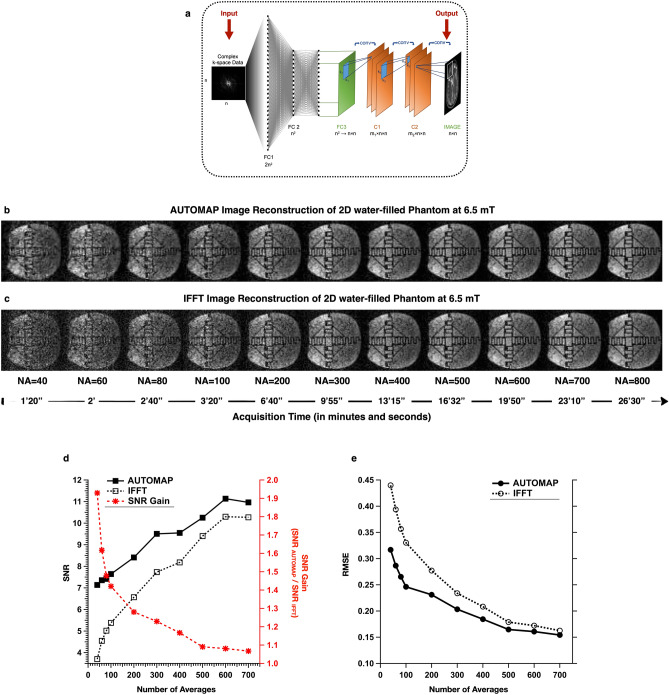
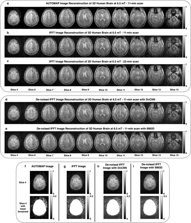
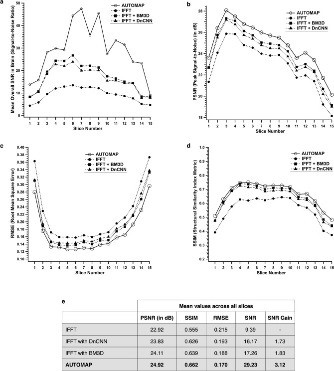
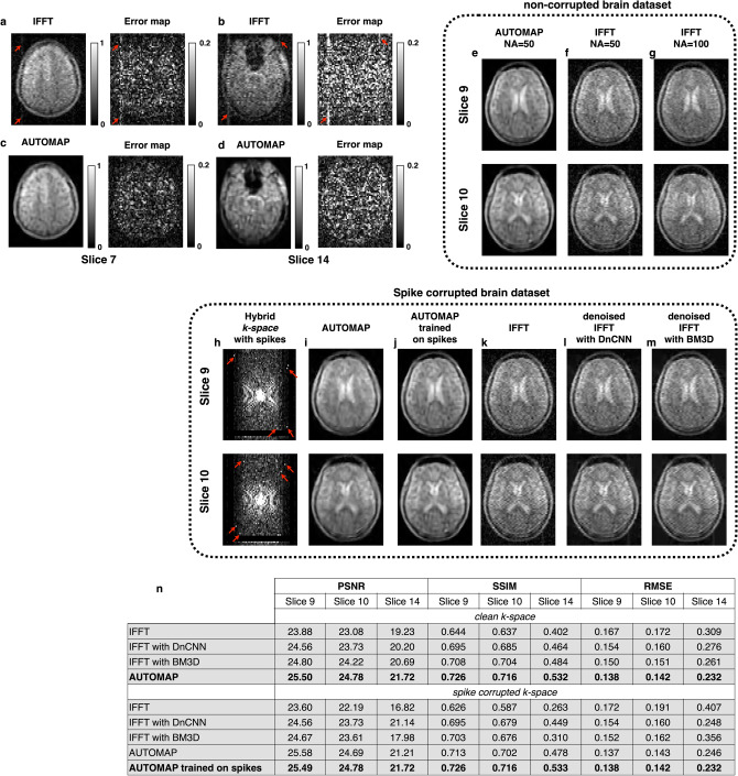
Recent years have seen a resurgence of interest in inexpensive low magnetic field (< 0.3 T) MRI systems mainly due to advances in magnet, coil and gradient set designs. Most of these advances have focused on improving hardware and signal acquisition strategies, and far less on the use of advanced image reconstruction methods to improve attainable image quality at low field. We describe here the use of our end-to-end deep neural network approach (AUTOMAP) to improve the image quality of highly noise-corrupted low-field MRI data. We compare the performance of this approach to two additional state-of-the-art denoising pipelines. We find that AUTOMAP improves image reconstruction of data acquired on two very different low-field MRI systems: human brain data acquired at 6.5 mT, and plant root data acquired at 47 mT, demonstrating SNR gains above Fourier reconstruction by factors of 1.5- to 4.5-fold, and 3-fold, respectively. In these applications, AUTOMAP outperformed two different contemporary image-based denoising algorithms, and suppressed noise-like spike artifacts in the reconstructed images. The impact of domain-specific training corpora on the reconstruction performance is discussed. The AUTOMAP approach to image reconstruction will enable significant image quality improvements at low-field, especially in highly noise-corrupted environments.

Figure 1

AUTOMAP neural network architecture and AUTOMAP image reconstruction at 6.5 mT—(a) the neural network architecture adapted from—the input to the network is the complex k-space data and the real and imaginary outputs are combined to form the final image. The network is comprised of two fully connected layers followed by two convolutional layers. (b,c) Comparison of AUTOMAP reconstruction with IFFT reconstruction for 2D imaging in a water-filled structured phantom—Images were acquired with a bSSFP sequence (matrix size = 64 × 64, TR = 31 ms at 6.5 mT. The number of signal averages (NA) increases from left to right with their respective scan time shown below. (b) Upper panel shows AUTOMAP-reconstructed images and (c) the lower panel shows same image reconstructed with IFFT. The window level of reconstructed images (b,c for each NA) is identical. (d) SNR Analysis of the 2D phantom dataset as a function of the different number of averages. The mean SNR versus NA is plotted on the left axis for AUTOMAP (filled square) and IFFT (open square). The SNR gain over IFFT is plotted (in red) on the right axis. (e) The Root Mean Square Error (RMSE) of the AUTOMAP reconstructed images (filled circle) and the IFFT reconstructed images (open circle) were evaluated with respect to the 800-average IFFT reconstructed image as reference.

Figure 2

3D brain image reconstruction at 6.5 mT using AUTOMAP compared to conventional IFFT with or without additional image-based denoising pipelines. (a–c) Reconstruction of 3D human head dataset—an 11-min (NA = 50) 3D acquisition dataset was reconstructed with AUTOMAP (a) and IFFT (b). Shown here are 10 slices from the full 15 slice dataset. For comparison, a 22-min (NA = 100) acquisition reconstructed with IFFT is shown in (c). The window level is unchanged in all images. (d,e) The two denoising algorithms (DnCNN and BM3D respectively) were applied to the IFFT reconstructed brain image (magnitude only) to compare to the denoising performance of AUTOMAP. (f–i) Noise floor comparison—Slice 4 from the NA = 50 reconstructed brain dataset shown above in (a,b) is displayed here with two different window levels: a normalized image on the top and a window level chosen to highlight the noise at the bottom. AUTOMAP is shown in (f), and IFFT is shown in (g). An additional DnCNN or BM3D image denoising step was applied to the image data reconstructed with IFFT (h,i respectively).

Figure 3

Image metric analysis on the 3D human brain dataset. (a–d) Image metric analysis of AUTOMAP and IFFT reconstruction with- and without the DnCNN step or the BM3D denoiser following transformation of the raw k-space data—The mean overall SNR in the whole-head ROI across all the 15 slices is shown in (a) for IFFT (filled circle), denoised IFFT with BM3D (filled square) with DnCNN (filled triangle), AUTOMAP (open circle). Three additional metrics are computed: PSNR (b), RMSE (c), and SSIM (d). (e) The table summarizes the mean PSNR, SSIM, RMSE, SNR and SNR gain values across all the slices. The SNR gain was calculated with respect to the conventional IFFT.

Figure 4

Artifacts: (a–d) Elimination of hardware artifacts at 6.5 mT—Two slices from a 3D bSSFP (NA = 50) are shown. When reconstructed with IFFT (a,b), a vertical artifact (red arrows) is present across slices. When the same raw data was reconstructed with AUTOMAP (c,d), the artifacts are eliminated. The error maps of each slice with respect to a reference scan (NA = 100) is shown for both IFFT and AUTOMAP reconstruction. (e–g) Uncorrupted k-space (NA = 50) was reconstructed with AUTOMAP (e) and IFFT (f). The reference NA = 100 scan is shown in (g). (h–m) AUTOMAP reconstruction of simulated k-space artifacts. Two slices of the hybrid k-space from the 11-min (NA = 50) brain scan was corrupted with simulated spikes (h). In (i), the data was reconstructed with AUTOMAP trained on the standard corpus of white Gaussian noise corrupted brain MRI images. In (j), the k-space data was reconstructed with AUTOMAP with a training corpus of k-space data including variable number of random spikes. IFFT reconstructed images are shown in (k), where the spiking artifacts are clearly seen. Denoised IFFT with DnCNN reconstructed images are shown in (I) and denoised IFFT with BM3D reconstructed images are shown in (m). (n) The table summarizes image quality metrics for the reconstruction task of the three slices, both with- and without spike corruption. PSNR, SSIM and RMSE were evaluated for reconstruction using IFFT, denoised IFFT with either DnCNN or BM3D, and AUTOMAP trained on either the standard Gaussian noise-corrupted corpus or on a spike- and Gaussian noise-corrupted corpus.

Figure 5

AUTOMAP is locally stable to noise: (a) histogram of the output-to-input variation ratio taken over noiseless- and Gaussian noise applied input data, with a low maximum value of 2.7. (b) histogram of the same output-to-input variation ratio taken over noiseless and Gaussian plus spike noise applied to the input data, with low maximum value of 1.5.

Figure 6

Domain-specific training corpora used on plant roots dataset—(a–c) Representative images from three training sets for root MRI reconstruction. (a) 2D images from the Human Connectome Project database. (b) 2D images from the training set based on synthetic vascular trees. Each of the 2D images was obtained by summing up the 3D synthetic vascular tree volumes in all 3 dimensions. (c) Images of realistic simulated root system from the RootBox toolbox. (d) The list of matrix sizes of the acquired root datasets and their corresponding training set used for image reconstruction.

Figure 7

Reconstruction of sorghum dataset acquired at 47 mT using AUTOMAP trained either on T₁-weighted MRI brain images, synthetic vascular tree Images, or synthetic root images. Six 2D projections of roots images (labelled dataset 1–6) extracted from six different roots’ samples are shown. All the 48 × 48 datasets were acquired at 47 mT. In the upper panel (a), the raw data were reconstructed with AUTOMAP trained on T₁-weighted MRI brain images, the panel (b) are the same datasets reconstructed with AUTOMAP trained on synthetic Vascular Tree Images and finally the same datasets were reconstructed with AUTOMAP trained on synthetic root images in panel (c). The lower panel (d) shows the images reconstructed with the standard IFFT method. All the images were windowed to the same level for comparison. The scale of 1 cm represented one of the images is the same for all the 2D projections. (e) The table summarizes the mean SNR analysis of the 2D projections of the roots 48 × 48 datasets acquired at 47 mT.

Figure 8

AUTOMAP reconstruction using the RootBox synthetic roots database versus IFFT reconstruction of a 96 × 96 root dataset. All eight 2D projections reconstructed with AUTOMAP are shown in (a), and with IFFT in (b). Each of the magnitude image was processed with either DnCNN as shown in the third panel (c) or with BM3D in the fourth panel (d) The window level for projections 1–7 were set to the same value except for projection 8, where the threshold was lowered on both panels to reveal the noise floor differences. To generate figure (e), the SNR was evaluated for AUTOMAP reconstruction using the RootBox training and compared to IFFT reconstruction with and without the denoising pipelines, and the SNR of each of the 8 projections reconstructed with AUTOMAP (open circle), IFFT without the denoising algorithm (filled circle), IFFT with BM3D (filled square), and IFFT with DnCNN (filled triangle) is plotted.

References

1. Waddington DEJ, Boele T, Maschmeyer R, Kuncic Z, Rosen MS. High-sensitivity in vivo contrast for ultra-low field magnetic resonance imaging using superparamagnetic iron oxide nanoparticles. Sci. Adv. 2020;6:eabb0998. doi: 10.1126/sciadv.abb0998. - DOI - PMC - PubMed
1. Marques JP, Simonis FFJ, Webb AG. Low-field MRI: an MR physics perspective. J. Magn. Reson. Imaging. 2019;49:1528–1542. doi: 10.1002/jmri.26637. - DOI - PMC - PubMed
1. Sarracanie M, et al. Low-cost high-performance MRI. Sci. Rep. 2015;5:15177. doi: 10.1038/srep15177. - DOI - PMC - PubMed
1. Sheth KN, et al. Assessment of brain injury using portable, low field magnetic resonance imaging at the bedside of critically Ill patients. JAMA Neurol. 2020 doi: 10.1001/jamaneurol.2020.3263. - DOI - PMC - PubMed
1. Ginde AA, Foianini A, Renner DM, Valley M, Camargo CA., Jr Availability and quality of computed tomography and magnetic resonance imaging equipment in U.S. emergency departments. Acad. Emerg. Med. 2008;15:780–783. doi: 10.1111/j.1553-2712.2008.00192.x. - DOI - PubMed
Publication types