The anisotropic field of ensemble coding

Abstract

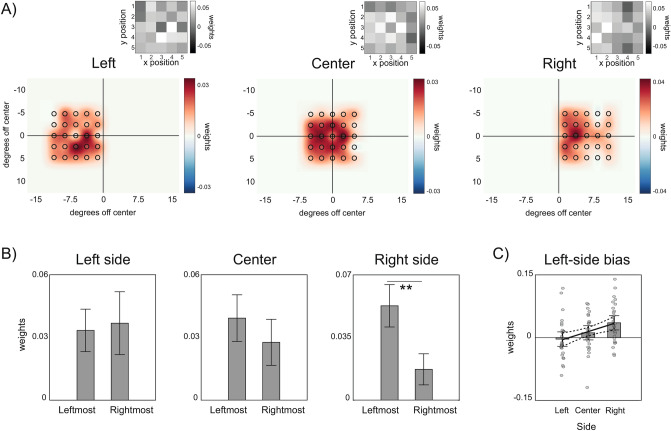
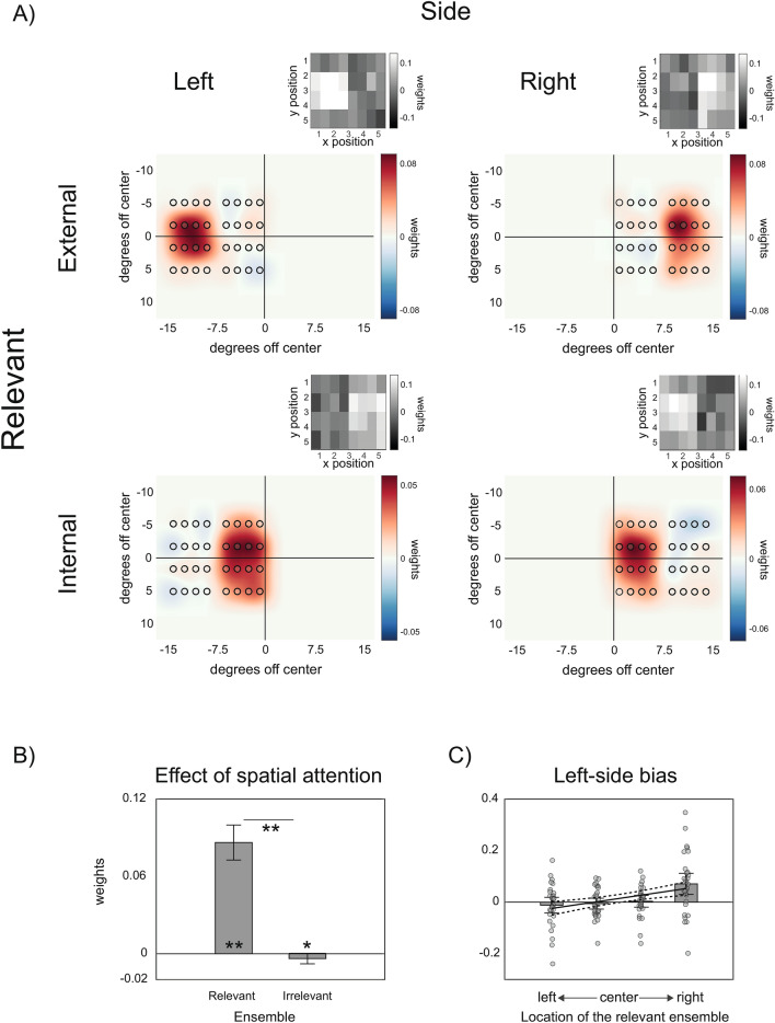
Human observers can accurately estimate statistical summaries from an ensemble of multiple stimuli, including the average size, hue, and direction of motion. The efficiency and speed with which statistical summaries are extracted suggest an automatic mechanism of ensemble coding that operates beyond the capacity limits of attention and memory. However, the extent to which ensemble coding reflects a truly parallel and holistic mode of processing or a non-uniform and biased integration of multiple items is still under debate. In the present work, we used a technique, based on a Spatial Weighted Average Model (SWM), to recover the spatial profile of weights with which individual stimuli contribute to the estimated average during mean size adjustment tasks. In a series of experiments, we derived two-dimensional SWM maps for ensembles presented at different retinal locations, with different degrees of dispersion and under different attentional demands. Our findings revealed strong spatial anisotropies and leftward biases in ensemble coding that were organized in retinotopic reference frames and persisted under attentional manipulations. These results demonstrate an anisotropic spatial contribution to ensemble coding that could be mediated by the differential activation of the two hemispheres during spatial processing and scene encoding.

Figure 1

Sequence of events in the ensemble coding tasks. (A) Example of one trial in Experiment 1. Stimuli were presented at the fovea with different degrees of dispersion (see “General methods” section). After the fixation cross, an ensemble of 25 disks was presented for 200 ms, followed by a blank interval. The task was to adjust the size (diameter) of a single central disk so that it reproduced the average size of the set of stimuli in the ensemble. (B) Example of one trial in Experiment 2, with the ensemble presented on the right side of the display. In this experiment, ensembles could randomly appear on the left, in the center or on the right side. (C) Example trial in Experiment 3. At the beginning of each trial, participants received a visual cue (here ‘IN’) indicating the region of the screen where the relevant ensemble was presented (here the internal region). After a fixation interval, two ensembles separated by colored frames were presented. Participants had to reproduce the average size of stimuli inside the relevant ensemble, indicated by a frame that matched the color of the initial cue. (D) Derivation of spatial weighting maps (SWMs). Local variations in the size of each disk across trials were used as multivariate regressors explaining the trial sequence of adjustment responses. Two-dimensional SWM were obtained by estimating the weight (regression coefficient) of each disk at each location on participants’ responses.

Figure 2

Results of Experiment 1. (A) SWM maps for each dispersion condition. Grey-scale maps visualize the original weights in matrix coordinates, estimated through the spatial weighted averaging model. Red and blue maps are the corresponding smoothed heatmaps, in screen coordinates. Histograms show the results of the permutation statistic, comparing the observed distance of weights ($\delta$) from a uniform distribution (black arrow) to that of randomly permuted surrogate maps (blue bars). (B) Comparison of weights along the vertical plane, collapsing columns of SWM maps. (C) Comparison of weights along the horizontal plane, collapsing rows of SWM maps. Error bars correspond to the standard deviation of the mean. * = p < 0.05; ** = p < 0.001.

Figure 3

Results of Experiment 2. (A) SWM maps for ensembles presented on the left side, center and right side of the screen. (B) Comparison of weights in the two leftmost and two rightmost columns of each condition, collapsing across the rows of the SWM maps. (C) Linear regression on the leftward bias (weights on two leftmost columns minus weights on two rightmost columns) as a function of the ensemble location, showing the increase of the bias from left to right.

Figure 4

Results of Experiment 3. (A) SWM maps for the four combinations of ensemble location (left and right) and relative position of the cued (relevant) ensemble (internal and external). (B) Overall weights assigned to stimuli in the relevant and irrelevant ensemble. (C) Linear regression on the leftward bias as a function of the actual location of the relevant ensemble.

References

1. Ariely D. Seeing sets: Representation by statistical properties. Psychol. Sci. 2001;12:157–162. - PubMed
1. Haberman J, Whitney D. Ensemble perception: Summarizing the scene and broadening the limits of visual processing. In: Wolfe J, Robertson L, editors. From Perception to Consciousness: Searching with Anne Treisman. Oxford University Press; 2012. pp. 339–349.
1. Whitney D, Leib AY. Ensemble perception. Annu. Rev. Psychol. 2018;69:105–129. - PubMed
1. Cohen MA, Dennett DC, Kanwisher N. What is the bandwidth of perceptual experience? Trends Cogn. Sci. 2016;20:324–335. - PMC - PubMed
1. Oliva A. Gist of the scene. In: Itti L, Rees G, Tsotsos JK, editors. Neurobiology of Attention. Elsevier; 2005. pp. 251–256.
Publication types
LinkOut - more resources