. 2021 Apr 15;11(1):8287.
doi: 10.1038/s41598-021-87881-w.

The image features of emotional faces that predict the initial eye movement to a face

Affiliations

The image features of emotional faces that predict the initial eye movement to a face

S M Stuit et al. Sci Rep. .

Abstract

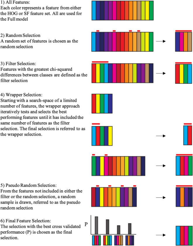
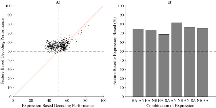
Emotional facial expressions are important visual communication signals that indicate a sender's intent and emotional state to an observer. As such, it is not surprising that reactions to different expressions are thought to be automatic and independent of awareness. What is surprising, is that studies show inconsistent results concerning such automatic reactions, particularly when using different face stimuli. We argue that automatic reactions to facial expressions can be better explained, and better understood, in terms of quantitative descriptions of their low-level image features rather than in terms of the emotional content (e.g. angry) of the expressions. Here, we focused on overall spatial frequency (SF) and localized Histograms of Oriented Gradients (HOG) features. We used machine learning classification to reveal the SF and HOG features that are sufficient for classification of the initial eye movement towards one out of two simultaneously presented faces. Interestingly, the identified features serve as better predictors than the emotional content of the expressions. We therefore propose that our modelling approach can further specify which visual features drive these and other behavioural effects related to emotional expressions, which can help solve the inconsistencies found in this line of research.


Conflict of interest statement

The authors declare no competing interests.

Figures

Figure 1
Figure 1
Visualisation of the Fourier feature extraction showing an example of two images used in a trial, their respective, down sampled Fourier features and the Fourier feature differences map. Note that in the Fourier Maps each location corresponds to a particular combination of a spatial frequency and an orientation. The Fourier maps are rotated 90° such that all have horizontal edge contrasts along the horizontal axes, and vertical edge contrast along the vertical axes. The radial axes are for cycles per image (abbreviated to cpi in the figure; ranging from low in the centre to high near the edges). Luminance intensity, from black to white, indicates the relative strength of the contrast for the corresponding section of the map. The Fourier feature differences map was calculated by subtracting the down sampled Fourier features of the image presented on the right, from those of the image on the left. Note that the feature difference map is scaled such that dark regions indicate negative values and light regions indicate positive values.
Figure 2
Figure 2
Visualisation of the HOG feature extraction showing an example of two images used in a trial, their respective HOG features and the HOG feature differences map using the highest resolution (10 × 10 cell size). All HOG maps use the same x and y axes as the original images, meaning position in the HOG map is directly coupled with position in an image. The HOG maps show 20 × 20 grids where each position in the grids represents an area of 10 × 10 pixels. For each 10 × 10 pixel area in an image, the weights for 9 differently oriented gradients are calculated. The 9 weights are visualized by white bars where the length reflects the weights. The 9 bars are then superimposed on the 10 × 10 pixel area there are based on. The HOG feature differences map was calculated by subtracting these HOG features weights of the image presented on the right, from those of the image on the left. Note that the feature difference map is scaled such that dark regions indicate negative values and light regions indicate positive values.
Figure 3
Figure 3
Schematic representation of the feature selection algorithm used in the current project. (1) Visual representation of the feature set. As a comparison to feature selection performance, all of the available features will be used to train and test a model referred to as the Full model. (2) A random collection of features (indicated by the red bars) is selected for a random selection. (3) The features are ranked based on Chi-Square scores. The top of the ranking is used to determine the filter model. (4) A search space is defined from the top-ranking features and the features in this search space are tested for inclusion into the wrapper selection through an iterative process until enough features have been selected for the wrapper model. (5) From the residual features, unused by the wrapper or filter selections, a random selection is made for a pseudo random selection. (6) Each of the four combinations of features are used to train classification models and cross-validation performance is subsequently estimated using the hold-out data. The final selection is based on highest cross-validation performance (P). See the above section Feature Inclusion, and the below section final feature selection for additional details.
Figure 4
Figure 4
The average percentage of initial eye movements, across participants, towards a particular expression (y-axis; HA happy, AN angry, NE neutral and SA sad) separately depending on the expression in the other image (x-axis). Note that this is for trials in which two different expressions were displayed. Results show a small but significant bias towards happy expressions. Figure generated using Matlab 2019b ( www.mathworks.com).
Figure 5
Figure 5
(A) The average decoding performance across participants (y-axis) for different modelling procedures (x-axis) based on the trials where different expressions were presented to the participants. (C) The same type of results but based on the trials where expressions have the same emotional content. The dotted lines represent the overall empirical chance level performance. Errorbars represent the standard error of the mean. (B,D) Confusion Matrices for the feature selection models. For all trials of each participant, we reorganized the decoding performance to show how well the model performed for combinations of expressions. Here, performance is represented as a matrix with expression of the right face on the y-axis and left face on the x-axis. Colour intensity reflects the fraction correct for the specific combination of expressions. Note that, performance is nearly equal for all combinations of expressions. Figures generated using Matlab 2019b ( www.mathworks.com).
Figure 6
Figure 6
Visual representations of the most relevant features for decoding. (A,B) Heatmaps (generated using MATLAB 2016a) reflecting the relevance of spatial locations of the HOG features to decoding either trials with different emotional content (A) or the same emotional content (B) overlaid on the averages of all images with a neutral expression. As relative importance of a location increases, colour changes from blue through green to yellow. (C) Here we show the weight, reflecting the percentage of contribution to overall performance, for each band of spatial frequencies used to decode face selection for both trial types (red line, different emotional content; green line same emotional content). Errorbars reflect the standard error of the mean. (D) Here we show the weight for each band of oriented edges used to decode initial eye movements for both trial types (red line, different emotional content; green line same emotional content). Errorbars reflect the standard error of the mean. Note that, for both spatial frequency and orientation, the only clear difference is a larger weight for horizontal orientations in trials where the emotional content differs. Figures generated using Matlab 2019b (www.mathworks.com).
Figure 7
Figure 7
Average decoding performances across all folds (y-axis) based on different sets of HOG and Fourier features. The dotted black lines represent chance level performance. Errorbars represent the standard error of the mean. (A) Average performance for decoding emotional content based on HOG features using three different feature sets at three different spatial resolutions (x-axis). EDf (Emotion Decoding features) uses a feature set based on feature selection for emotional content decoding, DETf (Different Emotion Trials features) uses the features based on decoding initial eye movements towards faces with different emotional content and SETf (Same Emotion Trials features) uses the features based on decoding initial eye movements towards faces with the same emotional content. (B) Average performance for decoding emotional content based on Fourier features, again using three different feature sets (x-axis). Note that, for both HOG and Fourier features, the features based on decoding initial eye movements are suboptimal for decoding emotional content. Moreover, only the high-resolution HOG features based on decoding eye movement behaviour are relevant for decoding emotional content.
Figure 8
Figure 8
(A) Relation between the average percentage correct prediction for each participant and each combination of emotions based on the biases towards expressions (x-axis) and the average corresponding percentage correct prediction based on the low-level image features of the images (y-axis). The dotted vertical line represents chance level performance for emotion-based decoding. The dotted horizontal line represents chance level performance for low-level image features-based decoding. The solid diagonal line shows where performance would be equal. (B) For each combination of emotions separately, the percentage of the predictions where low-level image features-based prediction out-performed prediction based on biases towards emotions. Note that for all emotions this is the case (all values well above 50%).

Similar articles

Cited by

References

    1. Parr LA, Winslow JT, Hopkins WD, de Waal F. Recognizing facial cues: individual discrimination by chimpanzees (Pan troglodytes) and rhesus monkeys (Macaca mulatta) J. Comp. Psychol. 2000;114(1):47. doi: 10.1037/0735-7036.114.1.47. - DOI - PMC - PubMed
    1. Burrows AM, Waller BM, Parr LA, Bonar CJ. Muscles of facial expression in the chimpanzee (Pan troglodytes): Descriptive, comparative and phylogenetic contexts. J. Anat. 2006;208(2):153–167. doi: 10.1111/j.1469-7580.2006.00523.x. - DOI - PMC - PubMed
    1. Darwin CR. The expression of emotions in man and animals. Philosophical Library; 1896.
    1. Ekman, P. (Ed.). (2006). Darwin and facial expression: A century of research in review. Ishk.
    1. Eibl-Eibesfeldt I. Foundations of human behavior. Human ethology. Aldine de Gruyter; 1989.

Publication types