

Eye-color and Type-2 diabetes phenotype prediction from genotype data using deep learning methods
- PMID: 33874881
- PMCID: PMC8056510
- DOI: 10.1186/s12859-021-04077-9
Eye-color and Type-2 diabetes phenotype prediction from genotype data using deep learning methods
Erratum in
-
Correction to: Eye‑color and Type‑2 diabetes phenotype prediction from genotype data using deep learning methods.BMC Bioinformatics. 2021 Jun 11;22(1):319. doi: 10.1186/s12859-021-04218-0. BMC Bioinformatics. 2021. PMID: 34116644 Free PMC article. No abstract available.
Abstract
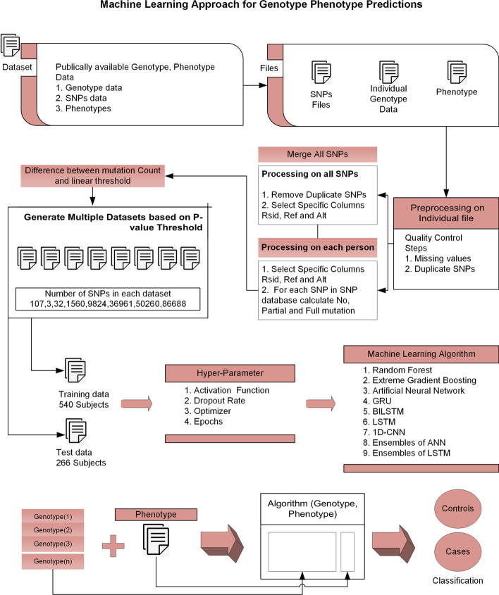
Background: Genotype-phenotype predictions are of great importance in genetics. These predictions can help to find genetic mutations causing variations in human beings. There are many approaches for finding the association which can be broadly categorized into two classes, statistical techniques, and machine learning. Statistical techniques are good for finding the actual SNPs causing variation where Machine Learning techniques are good where we just want to classify the people into different categories. In this article, we examined the Eye-color and Type-2 diabetes phenotype. The proposed technique is a hybrid approach consisting of some parts from statistical techniques and remaining from Machine learning.
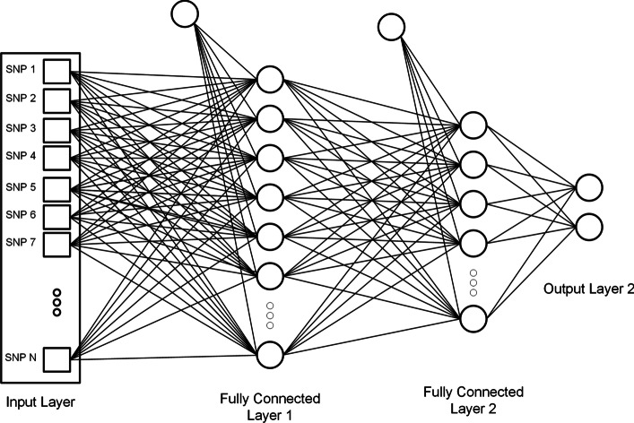
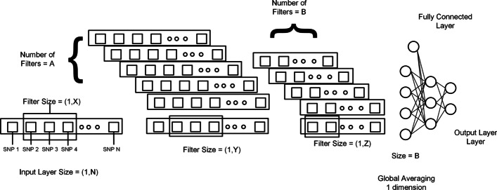
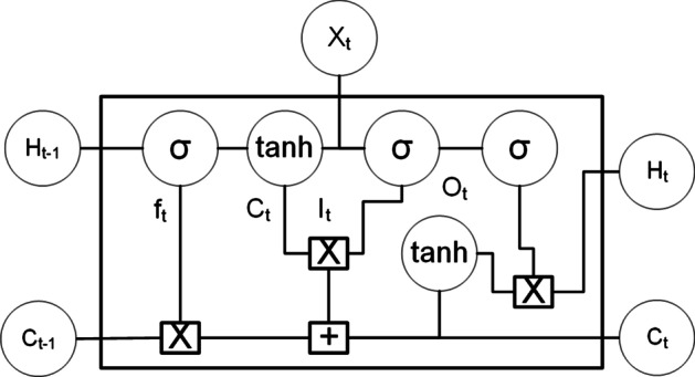
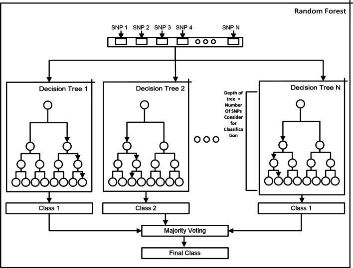
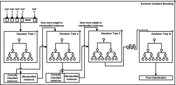
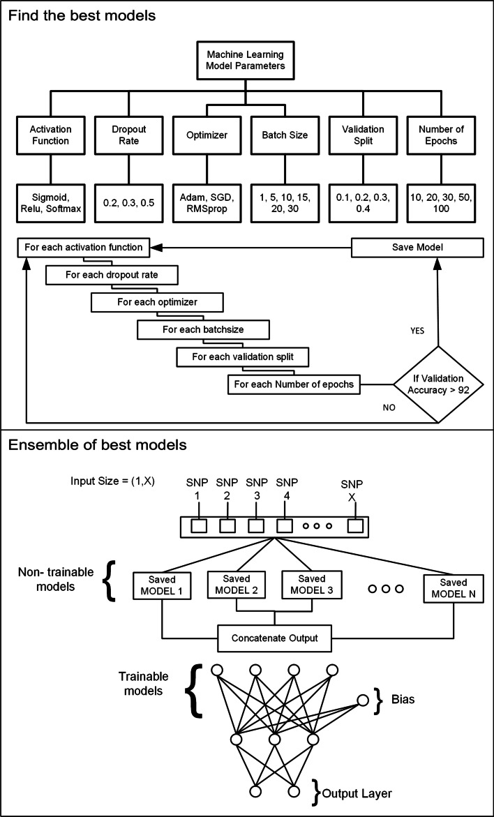
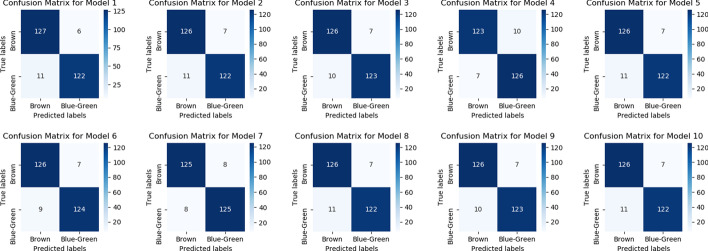
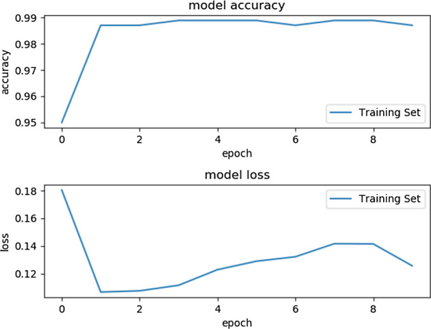
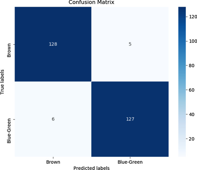
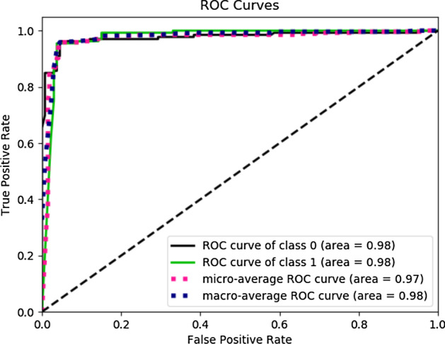
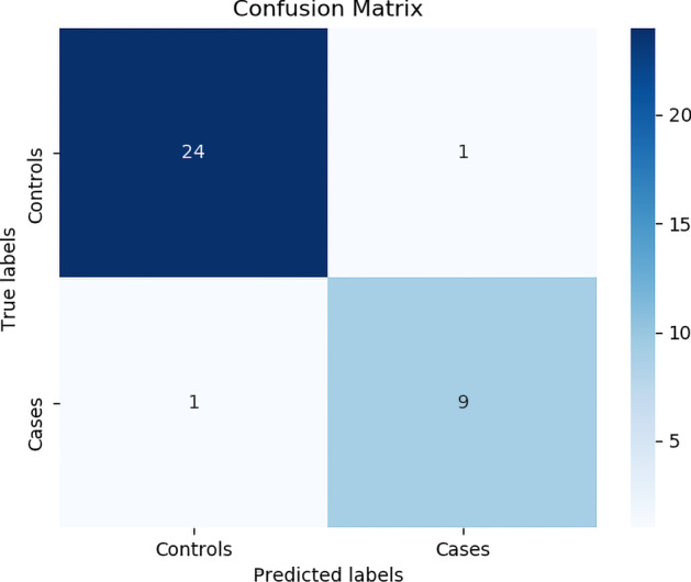
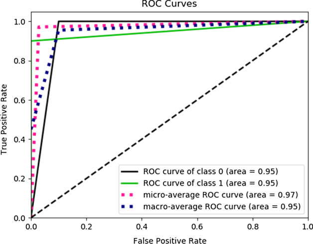
Results: The main dataset for Eye-color phenotype consists of 806 people. 404 people have Blue-Green eyes where 402 people have Brown eyes. After preprocessing we generated 8 different datasets, containing different numbers of SNPs, using the mutation difference and thresholding at individual SNP. We calculated three types of mutation at each SNP no mutation, partial mutation, and full mutation. After that data is transformed for machine learning algorithms. We used about 9 classifiers, RandomForest, Extreme Gradient boosting, ANN, LSTM, GRU, BILSTM, 1DCNN, ensembles of ANN, and ensembles of LSTM which gave the best accuracy of 0.91, 0.9286, 0.945, 0.94, 0.94, 0.92, 0.95, and 0.96% respectively. Stacked ensembles of LSTM outperformed other algorithms for 1560 SNPs with an overall accuracy of 0.96, AUC = 0.98 for brown eyes, and AUC = 0.97 for Blue-Green eyes. The main dataset for Type-2 diabetes consists of 107 people where 30 people are classified as cases and 74 people as controls. We used different linear threshold to find the optimal number of SNPs for classification. The final model gave an accuracy of 0.97%.
Conclusion: Genotype-phenotype predictions are very useful especially in forensic. These predictions can help to identify SNP variant association with traits and diseases. Given more datasets, machine learning model predictions can be increased. Moreover, the non-linearity in the Machine learning model and the combination of SNPs Mutations while training the model increases the prediction. We considered binary classification problems but the proposed approach can be extended to multi-class classification.
Keywords: Bioinformatics; Eye color; Genotype–phenotype; Machine learning; Type-2 diabetes.
Conflict of interest statement
The authors declare that they have no competing interests.
Figures
Similar articles
-
Further development of forensic eye color predictive tests.Forensic Sci Int Genet. 2013 Jan;7(1):28-40. doi: 10.1016/j.fsigen.2012.05.009. Epub 2012 Jun 17. Forensic Sci Int Genet. 2013. PMID: 22709892
-
Evaluation of the IrisPlex DNA-based eye color prediction assay in a United States population.Forensic Sci Int Genet. 2014 Mar;9:111-7. doi: 10.1016/j.fsigen.2013.12.003. Epub 2013 Dec 12. Forensic Sci Int Genet. 2014. PMID: 24528589
-
Performance of four models for eye color prediction in an Italian population sample.Forensic Sci Int Genet. 2019 May;40:192-200. doi: 10.1016/j.fsigen.2019.03.008. Epub 2019 Mar 11. Forensic Sci Int Genet. 2019. PMID: 30884346
-
Data-driven modeling and prediction of blood glucose dynamics: Machine learning applications in type 1 diabetes.Artif Intell Med. 2019 Jul;98:109-134. doi: 10.1016/j.artmed.2019.07.007. Epub 2019 Jul 26. Artif Intell Med. 2019. PMID: 31383477 Review.
-
Influenza virus genotype to phenotype predictions through machine learning: a systematic review.Emerg Microbes Infect. 2021 Dec;10(1):1896-1907. doi: 10.1080/22221751.2021.1978824. Emerg Microbes Infect. 2021. PMID: 34498543 Free PMC article.
Cited by
-
Can We Convert Genotype Sequences Into Images for Cases/Controls Classification?Front Bioinform. 2022 Jun 28;2:914435. doi: 10.3389/fbinf.2022.914435. eCollection 2022. Front Bioinform. 2022. PMID: 36304278 Free PMC article.
-
Transfer learning for genotype-phenotype prediction using deep learning models.BMC Bioinformatics. 2022 Nov 29;23(1):511. doi: 10.1186/s12859-022-05036-8. BMC Bioinformatics. 2022. PMID: 36447153 Free PMC article.
-
Development and validation of immune-based biomarkers and deep learning models for Alzheimer's disease.Front Genet. 2022 Aug 22;13:968598. doi: 10.3389/fgene.2022.968598. eCollection 2022. Front Genet. 2022. PMID: 36072674 Free PMC article.
-
Correction to: Eye‑color and Type‑2 diabetes phenotype prediction from genotype data using deep learning methods.BMC Bioinformatics. 2021 Jun 11;22(1):319. doi: 10.1186/s12859-021-04218-0. BMC Bioinformatics. 2021. PMID: 34116644 Free PMC article. No abstract available.
-
LSTM input timestep optimization using simulated annealing for wind power predictions.PLoS One. 2022 Oct 7;17(10):e0275649. doi: 10.1371/journal.pone.0275649. eCollection 2022. PLoS One. 2022. PMID: 36206213 Free PMC article.
References
-
- Basic genetics information—understanding genetics—NCBI bookshelf. https://www.ncbi.nlm.nih.gov/books/NBK115558/. Accessed 30 Nov 2020.
-
- Understanding genetics: a New York, mid-Atlantic guide for patients and health professionals—PubMed. https://pubmed.ncbi.nlm.nih.gov/23304754/. Accessed 30 Nov 2020. - PubMed
MeSH terms
LinkOut - more resources
Full Text Sources
Other Literature Sources
Medical
