An Overcomplete Approach to Fitting Drift-Diffusion Decision Models to Trial-By-Trial Data

Abstract

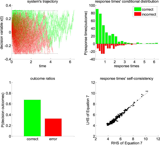
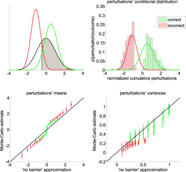
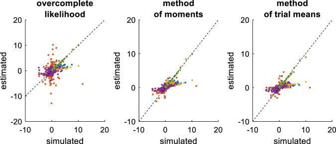
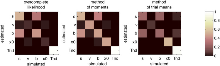
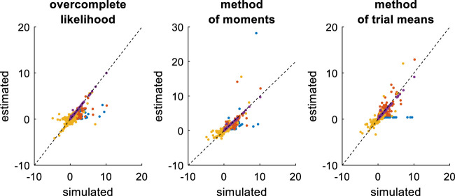
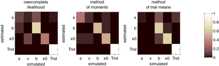
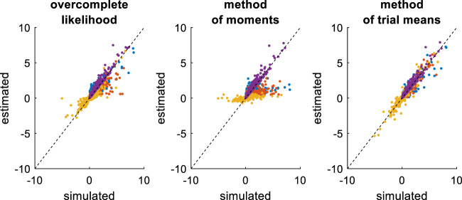
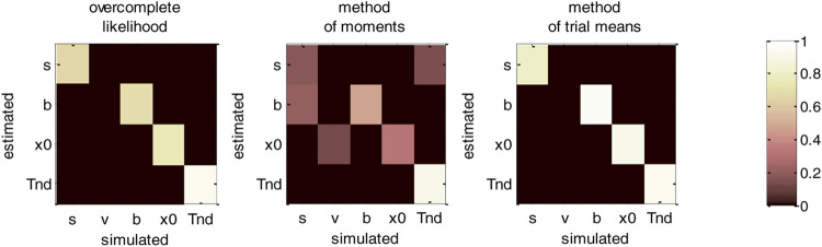
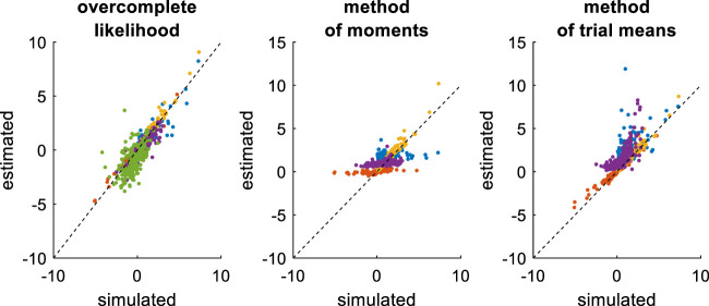
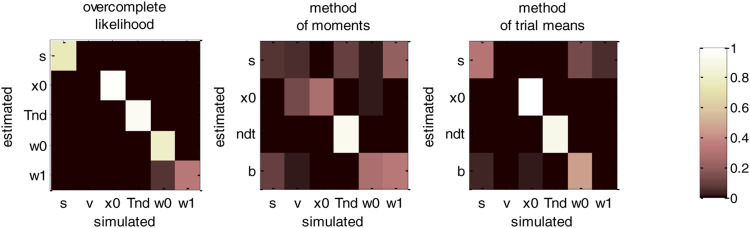
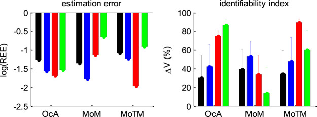
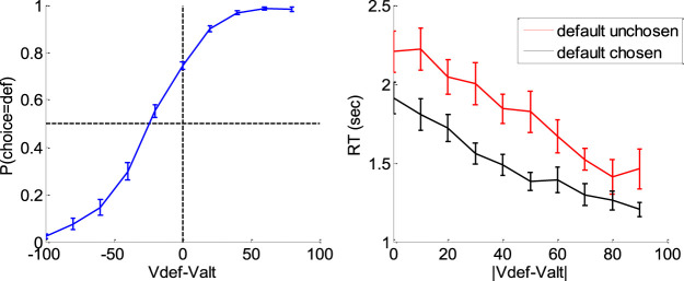
Drift-diffusion models or DDMs are becoming a standard in the field of computational neuroscience. They extend models from signal detection theory by proposing a simple mechanistic explanation for the observed relationship between decision outcomes and reaction times (RT). In brief, they assume that decisions are triggered once the accumulated evidence in favor of a particular alternative option has reached a predefined threshold. Fitting a DDM to empirical data then allows one to interpret observed group or condition differences in terms of a change in the underlying model parameters. However, current approaches only yield reliable parameter estimates in specific situations (c.f. fixed drift rates vs drift rates varying over trials). In addition, they become computationally unfeasible when more general DDM variants are considered (e.g., with collapsing bounds). In this note, we propose a fast and efficient approach to parameter estimation that relies on fitting a "self-consistency" equation that RT fulfill under the DDM. This effectively bypasses the computational bottleneck of standard DDM parameter estimation approaches, at the cost of estimating the trial-specific neural noise variables that perturb the underlying evidence accumulation process. For the purpose of behavioral data analysis, these act as nuisance variables and render the model "overcomplete," which is finessed using a variational Bayesian system identification scheme. However, for the purpose of neural data analysis, estimates of neural noise perturbation terms are a desirable (and unique) feature of the approach. Using numerical simulations, we show that this "overcomplete" approach matches the performance of current parameter estimation approaches for simple DDM variants, and outperforms them for more complex DDM variants. Finally, we demonstrate the added-value of the approach, when applied to a recent value-based decision making experiment.

Keywords: DDM; computational modeling; decision making; neural noise; variational bayes.

FIGURE 1

Impact of initial bias $x_0$. In all panels, the color code indicates the decision outcomes (green: “up” decisions, red: “down” decisions). The black dotted line indicates the default parameter value (for ease of comparison with other figures below). Upper-left panel: mean hitting times (y-axis) as a function of initial bias (x-axis). Upper-right panel: hitting times’ variance (y-axis) as a function of initial bias (x-axis). Lower-left panel: hitting times' skewness (y-axis) as a function of initial bias (x-axis). Lower-right panel: outcome ratios (y-axis) as a function of initial bias (x-axis).

FIGURE 2

Impact of drift rate $v$. Same format as Figure 1.

FIGURE 3

Impact of the perturbation’ standard deviation $\sigma$. Same format as Figure 1 (but the x-axis is now in log-scale).

FIGURE 4

Impact of the threshold’s height b. Same format as Figure 1.

FIGURE 5

Self-consistency equation. Monte-Carlo simulation of 200 trials of a DDM, with arbitrary parameters (in this example, the drift rate is positive). In all panels, the color code indicates the decision outcomes, which depends upon the sign of the drift rate (green: correct decisions, red: incorrect decisions). Upper-left panel: simulated trajectories of the decision variable (y-axis) as a function of time (x-axis). Upper-right panel: response times’ distribution for both correct and incorrect choice outcomes over the 200 Monte-Carlo simulations. Lower-left panel: outcome ratios. Lower-right panel: the left-hand side of Eq. 7 (y-axis) is plotted against the right-hand side of Eq. 7 (x-axis), for each of the 200 trials.

FIGURE 6

Approximate conditional distributions of the normalized cumulative perturbations. Upper-left panel: The black line shows the “no barrier” standard normal distribution of normalized cumulative perturbations. The shaded gray area has size $Q_{=}$, and its left bound (dashed black line) is the critical value ${\tilde{\eta }}_{=}$ below which cumulative perturbations eventually induce errors. The green and red lines depict the ensuing approximate conditional distributions given in Eq. 13. Upper-right panel: a Representative monte-carlo simulation. The green and red bars show the sample histogram of normalized cumulative perturbations for correct and erroneous decisions, respectively (over 200 trials, same simulation as in Figure 5). The green and red lines depict the corresponding approximate conditional normal distributions (cf. Eq. 13). Lower-left panel: The sample mean estimates of conditional perturbations (y-axis) are plotted against their “no barrier” approximation (x-axis, Eq. 11). Monte-carlo simulations are split according to the sign of the drift rate, and then binned according to deciles of approximate conditional means of normalized cumulative perturbations (green: Correct, red: error, errorbars: Within-decile means ± standard deviations). The black dotted line shows the identity mapping (perfect approximation). Lower-right panel: The sample variance estimates of normalized cumulative perturbations (y-axis) are plotted against their “no barrier” approximation (x-axis, Eq. 12). Same format as lower-left panel.

FIGURE 7

Comparison of simulated and estimated DDM parameters (full parameter set). Left panel: Estimated parameters using the overcomplete approach (y-axis) are plotted against simulated parameters (x-axis). Each dot is a monte-carlo simulation and different colors indicate distinct parameters (blue: $\sigma$, red: $v$, yellow: $b$, purple: $x_0$, green: $T_{ND}$). The black dotted line indicate the identity line (perfect estimation). Middle panel: Method of moments, same format as left panel. Right panel: Method of trial means, same format as left panel.

FIGURE 8

DDM parameter recovery matrices (full parameter set). Left panel: overcomplete approach. Middle panel: method of moments. Right panel: Method of trial means. Each line shows the squared partial correlation coefficient between a given estimated parameter and each simulated parameter (across 1000 Monte-Carlo simulations). Note that perfect recovery would exhibit a diagonal structure, where variations in each estimated parameter is only due to variations in the corresponding simulated parameter. Diagonal elements of the recovery matrix measure “correct estimation variability”, i.e., variations in the estimated parameters that are due to variations in the corresponding simulated parameter. In contrast, non-diagonal elements of the recovery matrix measure “incorrect estimation variability”, i.e., variations in the estimated parameters that are due to variations in other parameters. Strong non-diagonal elements in recovery matrices thus signal pairwise non-identifiability issues.

FIGURE 9

Comparison of simulated and estimated DDM parameters (fixed drift rates). Same format as Figure 7, except for the color code in upper panels (blue: $\sigma$, red: $b$, yellow: $x_0$, purple: $T_{ND}$).

FIGURE 10

DDM parameter recovery matrices (fixed drift rates). Same format as Figure 8, except that recovery matrices do not include the line that corresponds to the drift rate estimates. Note, however, that we still account for variations in the remaining estimated parameters that are attributable to variations in simulated drift rates.

FIGURE 11

Comparison of simulated and estimated DDM parameters (varying drift rates). Same format as Figure 9.

FIGURE 12

DDM parameter recovery matrices (varying drift rates). Same format as Figure 10, except that fixed drift rates are replaced by their average across DDM trials.

FIGURE 13

Comparison of simulated and estimated DDM parameters (collapsing bounds). Same format as Figure 9, except that the left panel includes an additional parameter ($w_1$: green color), which controls the decay rate of DDM bounds.

FIGURE 14

DDM parameter recovery matrices (collapsing bounds). Same format as Figure 12, except that recovery matrices now also include the bound’s decay rate parameter ($w_1$), in addition to the bound’s initial height ($w_0$).

FIGURE 15

Summary of DDM parameter recovery analyses. Left panel: The mean log relative estimation error $RRE$ (y-axis) is shown for all methods (OcA: Overcomplete approach, MoM: Method of moments, MoTM: Method of trial means), and all simulation series (black: Full parameter set, blue: fixed drift rate, red: varying drift rates, green: Collapsing bounds). Right panel: The mean identifiability index $\Delta V$ (y-axis) is shown for all methods and all simulation series (same format as left panel). Note that the situation in which the full parameter set has to be estimated serves as a References point. To enable a fair comparison, both the estimation error and the identifiability index are computed for the parameter subset that is common to all simulation series (i.e.: The perturbations ‘standard deviation $\sigma$, the bound’s height $b$, the initial condition $x_0$, and the non-decision time $T_{ND}$).

FIGURE 16

Evidence for choice and RT biases in the default/alternative frame. Left: Probability of choosing the default option (y-axis) is plotted as a function of decision value V_def-V_alt (x-axis), divided into 10 bins. Values correspond to likeability ratings given by the subject prior to choice session. For each participant, the choice bias was defined as the difference between chance level (50%) and the observed probability of choosing the default option for a null decision value (i.e., when V_def = V_alt). Right: Response time RT (y-axis) is plotted as a function of the absolute decision value |V_def-V_alt| (x-axis) divided into 10 bins, separately for trials in which the default option was chosen (black) or not (red). For each participant, the RT bias was defined as the difference between the RT intercepts (when V_def = V_alt) observed for each choice outcome.

FIGURE 17

Model-based analyses of choice and RT data. Left: For each participant, the observed choice bias (y-axis) is plotted as a function of the initial bias estimate ${\widehat{x}}_0$ in the default/alternative frame (x-axis). Right: Same for the observed RT bias.

References

1. Balci F., Simen P., Niyogi R., Saxe A., Hughes J. A., Holmes P., et al. (2011). Acquisition of decision making criteria: reward rate ultimately beats accuracy. Atten. Percept. Psychophys. 73, 640–657. 10.3758/s13414-010-0049-7 - DOI - PMC - PubMed
1. Beal M. J. (2003). Variational algorithms for approximate Bayesian inference/. PhD Thesis. London: University College London.
1. Bitzer S., Park H., Blankenburg F., Kiebel S. J. (2014). Perceptual decision making: drift-diffusion model is equivalent to a Bayesian model. Front. Hum. Neurosci. 8, 102. 10.3389/fnhum.2014.00102 - DOI - PMC - PubMed
1. Boehm U., Annis J., Frank M. J., Hawkins G. E., Heathcote A., Kellen D., et al. (2018). Estimating across-trial variability parameters of the diffusion decision model: expert advice and recommendations. J. Math. Psychol. 87, 46–75. 10.1016/j.jmp.2018.09.004 - DOI
1. Bogacz R., Brown E., Moehlis J., Holmes P., Cohen J. D. (2006). The physics of optimal decision making: a formal analysis of models of performance in two-alternative forced-choice tasks. Psychol. Rev. 113, 700–765. 10.1037/0033-295x.113.4.700 - DOI - PubMed
LinkOut - more resources