Extended Lattice Boltzmann Model

Abstract

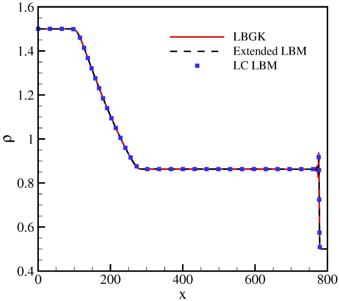
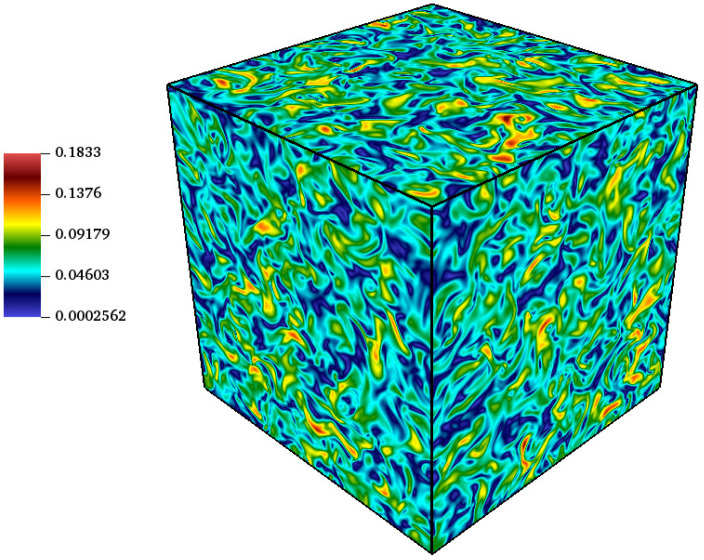
Conventional lattice Boltzmann models for the simulation of fluid dynamics are restricted by an error in the stress tensor that is negligible only for small flow velocity and at a singular value of the temperature. To that end, we propose a unified formulation that restores Galilean invariance and the isotropy of the stress tensor by introducing an extended equilibrium. This modification extends lattice Boltzmann models to simulations with higher values of the flow velocity and can be used at temperatures that are higher than the lattice reference temperature, which enhances computational efficiency by decreasing the number of required time steps. Furthermore, the extended model also remains valid for stretched lattices, which are useful when flow gradients are predominant in one direction. The model is validated by simulations of two- and three-dimensional benchmark problems, including the double shear layer flow, the decay of homogeneous isotropic turbulence, the laminar boundary layer over a flat plate and the turbulent channel flow.

Keywords: Galilean invariance; extended equilibrium; lattice Boltzmann method.

Figure A1

Spectral dissipation of acoustic modes for different models. Red symbols: LBGK; black symbols: extended LBM (33); blue symbols: LC LBM [9]; dashed line: Navier–Stokes. The velocity and temperature are set to $u_x=0.3$ and $T=T_L$.

Figure A2

Comparison of density profile for shock tube problem at density ratio ${\rho }_l/{\rho }_r=3$, after 500 iterations. Solid line: LBGK; dashed line: extended LBM (33); symbols: LC LBM [9].

Figure A3

Mach number profile, $\mathrm{Ma}=u/\sqrt{T_L}$, for the shock tube problem at density ratio ${\rho }_l/{\rho }_r=3$, after 500 iterations. Solid line: LBGK; dashed line: extended LBM (33); symbols: LC LBM [9].

Figure 1

Numerical measurement of viscosity for axis-aligned setup at temperature $T=1/3$ for different velocities. The exact solution corresponds to ${\nu }_{num}/\nu =1$.

Figure 2

Numerical measurement of viscosity for axis-aligned setup at Mach number $Ma=0.1$ for different temperatures. The exact solution corresponds to ${\nu }_{num}/\nu =1$.

Figure 3

Numerical measurement of viscosity for rotated setup at temperature $T=1/3$ for different velocities and stretching ratios. The exact solution corresponds to ${\nu }_{num}/\nu =1$.

Figure 4

Velocity magnitude in lattice units for the decaying homogeneous isotropic turbulence at ${\mathrm{Ma}}_{\mathrm{t}}=0.1$, ${\mathrm{Re}}_{\mathsf{\Lambda }}=72$ and $t^{*}=1.0$ with temperature $T=0.55$.

Figure 5

Time evolution of the turbulent kinetic energy for decaying isotropic turbulence at ${\mathrm{Ma}}_{\mathrm{t}}=0.1$, ${\mathrm{Re}}_{\mathsf{\Lambda }}=72$. Lines: present model; symbol: DNS [36].

Figure 6

Time evolution of the Taylor microscale Reynolds number for decaying isotropic turbulence at ${\mathrm{Ma}}_{\mathrm{t}}=0.1$, ${\mathrm{Re}}_{\mathsf{\Lambda }}=72$. Lines: present model; symbol: direct numerical simulations (DNS) [36].

Figure 7

Vorticity field for double shear layer flow at $t^{*}=1$ with regular lattice (left) and stretched lattice (right). Vorticity magnitude is normalized by its maximum value.

Figure 8

Evolution of kinetic energy (left) and enstrophy (right) for double shear layer flow at $Re={10}^4$.

Figure 9

Comparison of the velocity profile at $x=L_x$ for flow over a flat plate at different stretching ratios. Lines: present model; symbols: Blasius solution.

Figure 10

Comparison of the skin friction coefficient for flow over a flat plate at different stretching ratio. Lines: present model; symbols: analytical solution.

Figure 11

Snapshot of the velocity magnitude in lattice units for turbulent channel flow at ${\mathrm{Re}}_{\tau }=180$ with ${\lambda }_x=1.4$.

Figure 12

Comparison of the mean velocity profile in a turbulent channel flow at $R{e}_{\tau }=180$ with ${\lambda }_x=1.4$.

Figure 13

Comparison of the rms of the velocity fluctuations in a turbulent channel flow at $R{e}_{\tau }=180$ with ${\lambda }_x=1.4$. Symbols: present model; lines: DNS [40].

References

1. Succi S. The Lattice Boltzmann Equation: For Complex States of Flowing Matter. Oxford University Press; Oxford, UK: 2018.
1. Krüger T., Kusumaatmaja H., Kuzmin A., Shardt O., Silva G., Viggen E.M. The Lattice Boltzmann Method. Springer International Publishing; Cham, Switzerland: 2017.
1. Qian Y., Orszag S. Lattice BGK models for the Navier-Stokes equation: Nonlinear deviation in compressible regimes. EPL Europhys. Lett. 1993;21:255. doi: 10.1209/0295-5075/21/3/001. - DOI
1. Prasianakis N.I., Karlin I.V. Lattice Boltzmann method for thermal flow simulation on standard lattices. Phys. Rev. E. 2007;76:016702. doi: 10.1103/PhysRevE.76.016702. - DOI - PubMed
1. Prasianakis N.I., Karlin I.V. Lattice Boltzmann method for simulation of compressible flows on standard lattices. Phys. Rev. E. 2008;78:016704. doi: 10.1103/PhysRevE.78.016704. - DOI - PubMed
LinkOut - more resources