Dynamic patterns of correlated activity in the prefrontal cortex encode information about social behavior

Abstract

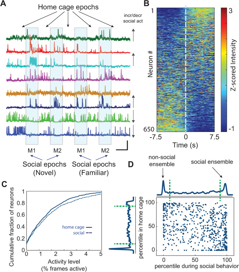
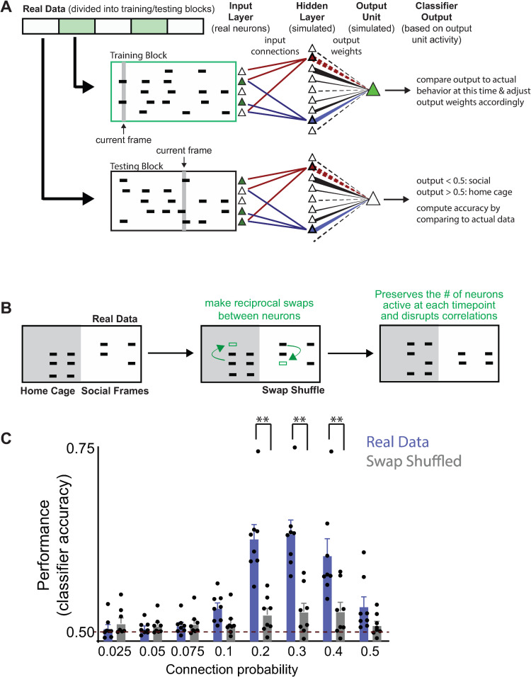
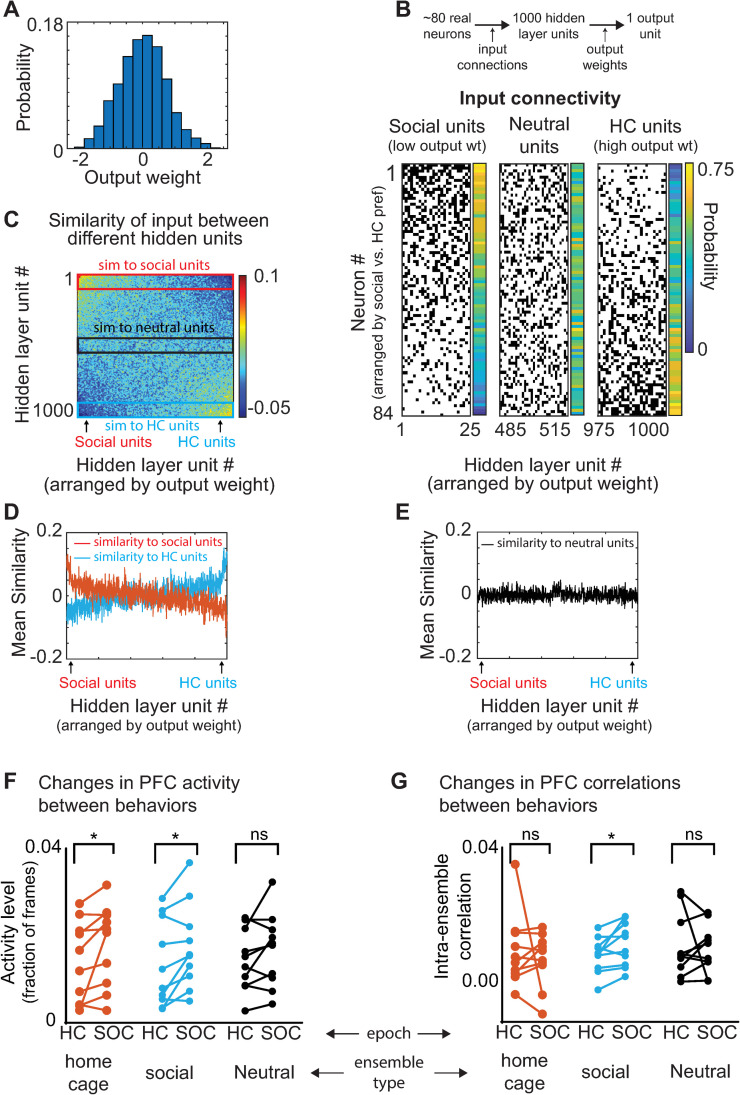
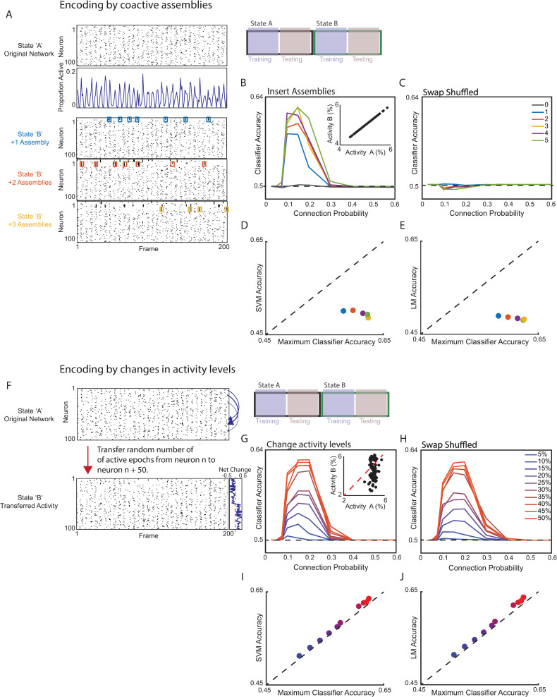
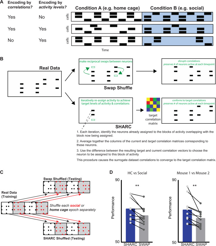
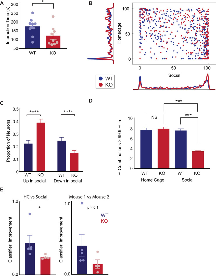
New technologies make it possible to measure activity from many neurons simultaneously. One approach is to analyze simultaneously recorded neurons individually, then group together neurons which increase their activity during similar behaviors into an "ensemble." However, this notion of an ensemble ignores the ability of neurons to act collectively and encode and transmit information in ways that are not reflected by their individual activity levels. We used microendoscopic GCaMP imaging to measure prefrontal activity while mice were either alone or engaged in social interaction. We developed an approach that combines a neural network classifier and surrogate (shuffled) datasets to characterize how neurons synergistically transmit information about social behavior. Notably, unlike optimal linear classifiers, a neural network classifier with a single linear hidden layer can discriminate network states which differ solely in patterns of coactivity, and not in the activity levels of individual neurons. Using this approach, we found that surrogate datasets which preserve behaviorally specific patterns of coactivity (correlations) outperform those which preserve behaviorally driven changes in activity levels but not correlated activity. Thus, social behavior elicits increases in correlated activity that are not explained simply by the activity levels of the underlying neurons, and prefrontal neurons act collectively to transmit information about socialization via these correlations. Notably, this ability of correlated activity to enhance the information transmitted by neuronal ensembles is diminished in mice lacking the autism-associated gene Shank3. These results show that synergy is an important concept for the coding of social behavior which can be disrupted in disease states, reveal a specific mechanism underlying this synergy (social behavior increases correlated activity within specific ensembles), and outline methods for studying how neurons within an ensemble can work together to encode information.

Fig 1. Social interaction modulates activity levels within prefrontal ensembles.

(A) Mice were imaged across 9 consecutive behavioral epochs (each lasting 5 minutes) during which they were either alone in their HC or interacted with one of 2 novel sex-matched juvenile mice introduced to the HC (“M1” or “M2”). Each novel mouse was subsequently reintroduced to the HC during a familiar epoch. GCaMP traces show examples of neurons that appear to increase or decrease activity during social epochs (see arrows at the right of each trace). Scale bar: x-axis represents 5 minutes, and y-axis denotes maximum dF/F₀ for each trace (scaled independently). (B) Mean z-scored GCaMP traces for all neurons recorded from WT mice (663 neurons from 10 mice) aligned to the onset of social interaction during the first bout of interaction within each social epoch. (C) Cumulative plot showing the distribution of activity levels for individual neurons during HC epochs or periods of social interaction (% time active in HC: 1.8 +/− 0.1%, % time active during social interaction: 2.1 +/− 0.1%, p = 0.00002, paired t test; n = 663 neurons from 10 WT mice). (D) Scatter plot showing the activity of each neuron during each behavioral condition, expressed as a percentile relative to a null distribution generated by circularly shuffling that neuron’s activity. Activity levels during social interaction or while the mouse was alone in its HC are plotted on the x-axis and y-axis, respectively. Kernel density plots along the axes indicate the fraction of neurons whose activity was at a given percentile of the null distribution. Neurons with activity >90th percentile of shuffled datasets (green dotted line) were considered to be positively modulated, whereas neurons with activity <10th percentile (green dotted line) were considered to be negatively modulated during each behavior (>90th percentile, social: 152/663 neurons, HC: 80/663 neurons; p < 0.00001, chi-squared test; <10th percentile, social: 128/663 neurons, HC: 119/663 neurons; p = 0.5, chi-squared test). Data used to generate this figure can be found in the Supporting information Excel spreadsheet (S1 Data). HC, home cage; WT, wild-type.

Fig 2. Classifying behavior from prefrontal ensembles using a simple neural network.

(A) We constructed a neural network consisting of a single hidden layer (containing 1,000 units) connected to a single output unit. The thickness of lines between each hidden layer unit and the output unit reflects the magnitude of the output weight. Positive and negative weights are indicated by solid and dashed lines, respectively. Each hidden layer unit received input from a random subset of prefrontal neurons from one real dataset. For clarity, we have only shown input connections to 2 hidden layer units (which are differentiated by their blue and red colors)—output weights from other hidden units are shown in black. The output weight from each hidden layer unit was iteratively updated during training. We trained the classifier to distinguish periods marked as HC exploration or social interaction by dividing a dataset into 500-frame blocks and then using alternating blocks for training or testing. (B) Cartoon describing swap shuffling procedure. Note that in this figure, we swapped events between neurons and across the entire dataset, thereby disrupting behavior-specific changes in the activity levels of individual neurons, while preserving both the total activity for each neuron (over the entire experiment) and the number of neurons active in any given frame. (C) The classifier performed poorly (near chance) when the input connection probability (governing the number of prefrontal neurons that provided input to each hidden layer unit) was <10%. Classification accuracy was above chance in 8/10 mice and increased to a peak of 69 +/− 3% in these mice, before decreasing again for connection probabilities >30%. The classifier performance was significantly decreased to near-chance levels when we trained and tested using data that had been randomly swap shuffled (2 way RM ANOVA shuffle vs. real p < 0.0005; connection p < 0.0001, interaction p < 0.0001; follow-up with Bonferonni multiple comparisons test revealed significant differences for input connection probabilities of 20%, 30%, and 40% at p < 0.01). Data used to generate this figure can be found in the Supporting information Excel spreadsheet (S1 Data). HC, home cage; RM ANOVA, repeated measures analysis of variance.

Fig 3. Classifier weights reveals an ensemble that increases correlations during social behavior and detects social behavior.

(A) Example histogram depicting the distribution of output weights assigned to connections between hidden layer units and the output unit over the course of training. (B) Matrix of input connections for hidden units which detect the social (left) or HC condition (right). The hidden layer units (x-axis) have been arranged in order of increasing output weights to identify “social units” (25 most negative output weights) and “HC units” (25 largest positive output weights). We also plotted “neutral units” (30 units closest to 0). To the right of each matrix is the probability that a given neuron will be connected to a given set of units. Prefrontal neurons (y-axis) have been arranged in order of their preference for social interaction vs. HC, i.e., the difference in their probability of being connected to home cage versus social units. (C) Correlation matrix showing the input similarity, i.e., the pairwise correlation between binary vectors representing the input connections to each pair of hidden layer units. Hidden layer units are arranged in order of increasing output weight. Red and blue rectangles indicate the input similarity compared to social or HC units, respectively. A Gaussian filter with a standard deviation of 3 was applied to the 1,000 × 1,000 matrix to improve visualization. (D) For each hidden layer unit, we plotted its average input similarity to either the 25 social units (red) or the 25 HC units (blue). Hidden layer units (x-axis) are again arranged by output weight. Social units had similar patterns of input compared to each other but not to HC units and vice versa. (E) The average input similarity of each hidden layer unit to 25 hidden layer units with near-zero output weights (“neutral units”; black rectangle in C). (F) We defined social and HC ensembles as the 20% of prefrontal neurons most likely to provide input to the social or HC units, respectively. The mean activity of both HC and social ensembles increased during social interaction compared to the HC condition (social ensemble: mean activity level 1.4 +/− 0.3% in HC vs. 1.8 +/− 0.3% during social interaction, p < 0.05, sign-rank test; HC ensemble: mean activity level 1.5 +/− 0.30% in HC vs. 1.9 +/− 0.3% during interaction, p < 0.001, sign-rank test; neutral ensemble 1.5 +/− 0.2 in HC vs. 1.7+/− 0.3 during interaction, p = 0.16). (G) Correlations between neurons in the same ensemble increased during social interaction for the social ensemble (mean correlation between neurons in the social ensemble: 0.008 +/− 0.002 in HC vs. 0.012 +/− 0.002 during social interaction, p < 0.05; HC ensemble mean correlation 0.010 +/− 0.003 in HC vs. 0.007 +/− 0.003 during social interaction, p = 0.77, sign-rank test; neutral ensemble mean correlation coefficient 0.011 +/− 0.003 in HC vs. 0.010 +/− 0.002 during social interaction; p = 0.7). Note: A–E show a representative example from a single mouse. F and G represent data from a single iteration of the classifier at the optimal input connection probability (0.3) averaged over all mice. Data used to generate this figure can be found in the Supporting information Excel spreadsheets (S1 Data for panels F and G and S2 Data for panels C–E). HC, home cage; PFC, prefrontal cortex.

Fig 4. Neural network classifiers can distinguish states which differ in either activity or correlations.

(A) We generated synthetic datasets consisting of 100 neurons. Each dataset consisted of 2 activity rasters, corresponding to States “A” and “B.” Each raster contained 6,000 time points (frames). The overall level of activity in each raster oscillated around a mean level (5% of neurons active in a frame). In “State A,” neuronal activity was randomly assigned. Then, we created 1–5 cell assemblies in “State B” by rearranging the activity raster for “State A.” Specifically, whenever the first neuron in an assembly was active, we swapped activity across the rest of the network so that other neurons in the same assembly would be coactive. This was achieved by making reciprocal swaps between neurons. For example, suppose a neuron outside the assembly was active in the desired frame. Then, we swapped its activity with a neuron within the assembly that was active in a different frame. Thus, neither the total number of neurons active in a given frame nor the total activity level of any neuron differed between the “State A” and “State B” rasters. As a result, “State B” was differentiated from “State A” only by the presence of 1, 2, 3, 4, or 5 assemblies comprised of correlated (coactive) neurons. (B) A neural network classifier performed above chance in distinguishing “State A” from “State B” (50% of the data was used for training and the remainder for testing). For each level of coactivity (1, 2, 3, 4, or 5 assemblies), performance was averaged over 5 different “State A” rasters and 4 unique “State B” rasters for each “State A” raster. As a control, the dark gray trace shows mean classifier performance when “State B” was replaced with a second randomly generated template containing 0 inserted assemblies. Inset shows the activity level of each neuron in “State A” plotted against its activity level in “State B.” (C) The classifier, trained on the original “State A” and “State B” rasters, performed at chance levels when tested on swap-shuffled versions of the “State A” and “State B” rasters. Swap shuffling each raster destroys correlated patterns of activity. (D) Scatter plot comparing accuracy of a linear SVM classifier to the optimal performance of our neural network classifier. In both cases, 50% of the data was used for training and the remainder for testing. Each dot represents the average of 4 simulations using the indicated number of inserted assemblies. (E) Scatter plot comparing accuracy of classification using logistic regression to the optimal performance of our neural network classifier. In both cases, 50% of the data was used for training and the remainder for testing. Each dot represents the average of 4 simulations using the indicated number of inserted assemblies. (F) We generated synthetic datasets which differ in activity levels. The “State A” rasters were as described in panel A. In this case, “State B” rasters were generated by transferring a proportion of the activity from the first 50 neurons in each State A raster to neurons 51–100. In this manner, half the neurons increased their activity in “State B” compared to “State A”; the other half decreased. The proportion of activity transferred was determined by randomly drawing a number with an upper bound ranging from 5% to 50%. (G) We used 50% of the data to train a neural network classifier to distinguish “State A” from “State B.” The remaining data were used for testing. Insert shows the activity level of each neuron in “State A” plotted against its activity in “State B.” The color of the trace indicates the max % of activity that was shifted from neurons 1–50 to neurons 51–100 when generating the State B raster. (H) Swap shuffling each raster (preserving differences in the activity levels of individual neurons between States A and B while disrupting correlations) does not decrease classification accuracy. (I) Scatter plot comparing the accuracy of a linear SVM classifier to the optimal performance of our neural network classifier. For both classifiers, 50% of the data was used for training and the remainder for testing. Each dot represents the average of 4 simulations, and the color indicates the maximum amount of activity transferred from neurons 1–50 to neurons 51–100. (J) Scatter plot comparing the accuracy of logistic regression to the optimal performance of our neural network classifier. For both classifiers, 50% of the data was used for training and the remainder for testing. Each dot represents the average of 4 simulations, and the color indicates the maximum amount of activity transferred from neurons 1–50 to neurons 51–100. Data used to generate this figure can be found in the Supporting information Excel spreadsheet (S1 Data). SVM, support vector machine; LM, linear model (logistic regression).

Fig 5. Correlations transmit additional information beyond that conveyed by changes in activity levels.

(A) Cartoon illustrating that information about behavior may be encoded through changes in activity levels, correlations between neurons, or both. (B) To disentangle the roles of activity levels and correlations in transmitting information, we used 2 different methods to create shuffled (surrogate) datasets which preserve changes in activity levels, but either do or do not preserve patterns of correlations. We made random, reciprocal swaps of activity between neurons to generate surrogate datasets which maintained network activity in each frame as well as the number of blocks of activity for each neuron. However, this swap shuffling destroyed the correlation structure. In a second set of surrogate datasets, we used SHARC to iteratively generate surrogates in which the correlation structure was also maintained. (C) To maintain behavior-specific changes in activity levels and correlations that are associated with the 2 behavioral conditions, we swap shuffled or performed SHARC separately for each behavioral epoch, then concatenated the 9 resulting surrogate subrasters to create each surrogate dataset. (D) We trained a neural network classifier (using input connection probability = 0.3) on each real dataset, then tested that classifier on swap or SHARC-shuffled surrogate datasets generated from that real dataset. Accuracy was significantly higher for the SHARC-shuffled surrogates, which maintain the behaviorally modulated correlations found in the original dataset. Left: accuracy for surrogate datasets in classifying periods of HC vs. SOC behavior = 71 +/− 2 (SHARC) vs. 67 +/− 2% (swap), p = 0.005, paired t test. Right: accuracy for surrogate datasets in classifying interaction with Mouse 1 vs. interaction with Mouse 2: 71 +/− 3% (SHARC) vs. 65 +/− 2% (swap), p = 0.007, paired t test. n = 10 mice. Data used to generate this figure can be found in the Supporting information Excel spreadsheet (S1 Data). HC, home cage; SHARC, SHuffling Activity to Re-arrange Correlations; SOC, social.

Fig 6. Shank3 KO mice have disorganized ensembles for which correlations fail to enhance the transmission of information about social behavior.

(A) The mean time that Shank3 KO mice or WT littermates spend interacting with a novel juvenile mouse of the same sex during a 5-minute assay. Data have been pooled from 8 unimplanted WT mice as well as the 5 implanted WT mice used for microendoscopic imaging and 5 unimplanted KO mice in addition to the 4 implanted mice used for imaging. For implanted mice, we used the average of interaction time for the 2 novel mice. Pooled data showed decreased interaction in KO mice (173 +/− 12 seconds vs. 120 +/− 18 seconds for WT and KO respectively, p < 0.05, t test). The unimplanted cohort alone shows a similar significant decrease in interaction time for KO mice (165 +/− 15 seconds vs. 110 +/− 16 seconds for WT and KO respectively, p < 0.05, t test). In the implanted cohort, there was a similar trend toward decreased interaction for KO mice (186 +/− 20 seconds vs. 133 +/− 37 seconds for WT and KO respectively, p = 0.21, t test). (B) (Similar to Fig 1D). Scatter plot showing the activity of each neuron during each behavioral condition, expressed as a percentile relative to a null distribution generated by circularly shuffling that neuron’s activity. Activity levels during social interaction or while the mouse was alone in its HC are plotted on the x-axis and y-axis, respectively. Kernel density plots along the axes indicate the fraction of neurons whose activity was at a given percentile of the null distribution. Neurons with activity >90th percentile of shuffled datasets (green dotted line) were considered to be positively modulated, whereas neurons with activity <10th percentile (green dotted line) were considered to be negatively modulated during each behavior. Data are plotted for Shank3 KO mice (red) and WT littermates (blue) (mean percentile of activity during social interaction, WT: 50 +/− 2 percentile; KO: 64 +/− 2 percentile; p < 0.0001 by 2-sample t test; mean percentile of activity during HC, WT: 47 +/− 2 percentile; KO: 51 +/− 2 percentile; p = 0.1, t test). (C) Bar graph showing the fraction of neurons whose activity was positively or negatively modulated (>90th percentile or <10th percentile) during social interaction. The proportion of neurons which increased activity during social interaction was significantly greater in KO mice (22% in WT vs. 39% in KO, chi-squared = 17.7, p < 0.0001), whereas the down-regulated ensemble was significantly smaller in KO mice (25% in WT vs. 15% in KO, chi-squared test, 8.2, p < 0.005). Error bars denote the binomial SEM algebraically derived from total number of neurons and the proportion that were modulated in the specified direction. (D) The proportion of 3-neuron combinations occurring during HC exploration that are enriched >99.9th percentile compared to swap-shuffled datasets was similar across WT (blue; 7.6%) and KO (red; 7.8%) mice. By contrast, the proportion of 3-neuron combinations occurring during social interaction that are enriched >99.9th percentile compared to swap-shuffled datasets was 7.5% in WT compared to only 3.4% in KO mice (total number of HC combinations: 4,187 in 5 WT mice and 5,878 in 4 KO mice; total number of social combinations: 5,487 in 5 WT mice and 16,326 in 4 KO mice). We have plotted this data as a bar graph showing the fraction of these combinations that were specifically enriched above the 99.9th percentile (chi-squared = 165, p < 0.0001). Error bars denote the SEM algebraically derived from the binomial distribution, the number of 3-neuron combinations in each condition, and the proportion of those combinations that were enriched. (E) Bar graph showing how much better classifiers trained on real datasets perform when tested on SHARC-shuffled datasets, compared to their performance when tested on swap-shuffled datasets, i.e., (PerformanceSHARC – PerformanceSwap)/(PerformanceSwap − 0.5). Each datapoint represents a classifier from one mouse. Left: The increase in performance was significantly larger in WT mice (blue) than KO mice (right) for classification of HC periods (HC) vs. epochs of social interaction (Social), WT: 0.44 +/− 0.10 vs. KO: 0.24 +/− 0.01, p = 0.016, Mann–Whitney. Right: The increase in performance was nonsignificantly larger in WT mice (blue) than KO mice (right) for classification of interactions with Mouse 1 vs. those with Mouse 2, WT: 0.41 +/− 0.15 vs. KO: 0.14 +/− 0.06, p = 0.11, Mann–Whitney. Combined analysis of both classifications (HC vs. Soc and Mouse 1 vs. Mouse 2) shows a significant effect of genotype: p < 0.05 by 2-way ANOVA. Data used to generate this figure can be found in the Supporting information Excel spreadsheet (S1 Data). HC, home cage; KO, knockout; SHARC, SHuffling Activity to Re-arrange Correlations; WT, wild-type.

References

1. Cai DJ, Aharoni D, Shuman T, Shobe J, Biane J, Song W, et al.. A shared neural ensemble links distinct contextual memories encoded close in time. Nature. 2016. 10.1038/nature17955 - DOI - PMC - PubMed
1. Liang B, Zhang L, Barbera G, Fang W, Zhang J, Chen X, et al.. Distinct and Dynamic ON and OFF Neural Ensembles in the Prefrontal Cortex Code Social Exploration. Neuron [Internet]. 2018. November 7 [cited 2019 Mar 30];100(3):700–14.e9. Available from: https://www.sciencedirect.com/science/article/pii/S0896627318307724?via%... 10.1016/j.neuron.2018.08.043 - DOI - PMC - PubMed
1. deCharms RC, Merzenich MM. Primary cortical representation of sounds by the coordination of action-potential timing. Nature [Internet]. 1996. June 13 [cited 2019 Aug 25];381(6583):610–3. Available from: http://www.ncbi.nlm.nih.gov/pubmed/8637597 10.1038/381610a0 - DOI - PubMed
1. Hebb DO. The organization of behavior: A neuropsychological theory. New York: Wiley; 1949.
1. Buzsáki G. Neural Syntax: Cell Assemblies, Synapsembles, and Readers. Neuron [Internet]. 2010. November 4 [cited 2019 Mar 30];68(3):362–85. Available from: http://www.ncbi.nlm.nih.gov/pubmed/21040841 10.1016/j.neuron.2010.09.023 - DOI - PMC - PubMed
Publication types