Individual-Specific Areal-Level Parcellations Improve Functional Connectivity Prediction of Behavior

Abstract

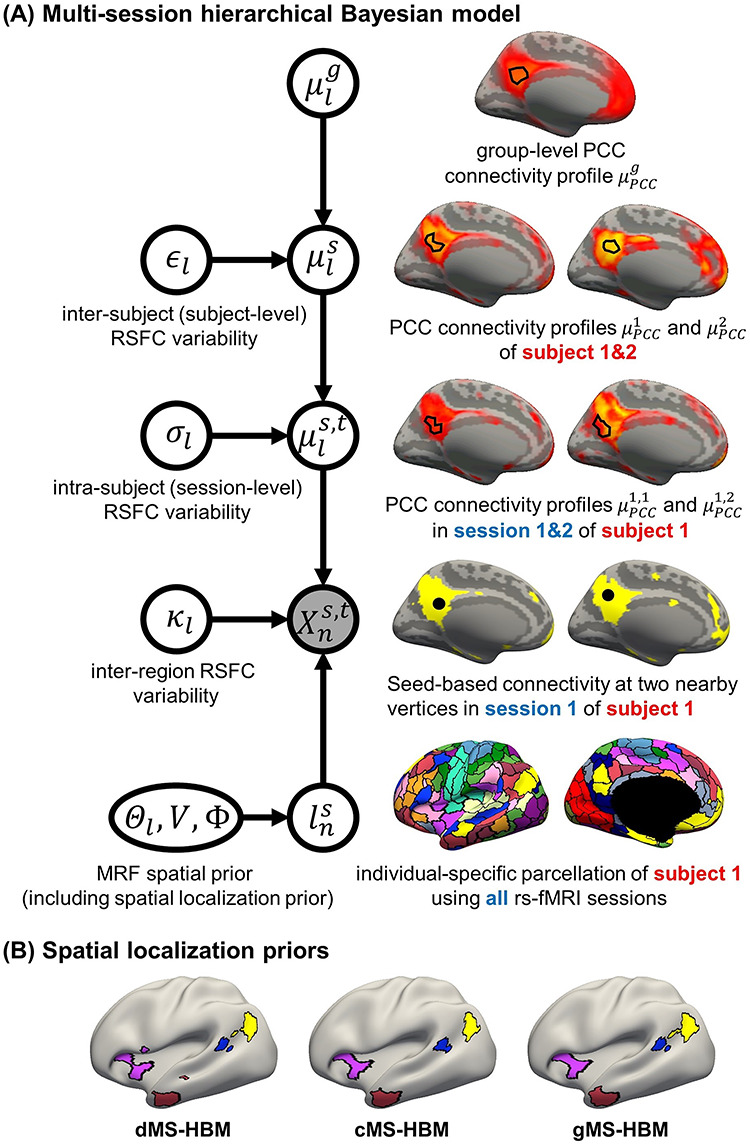
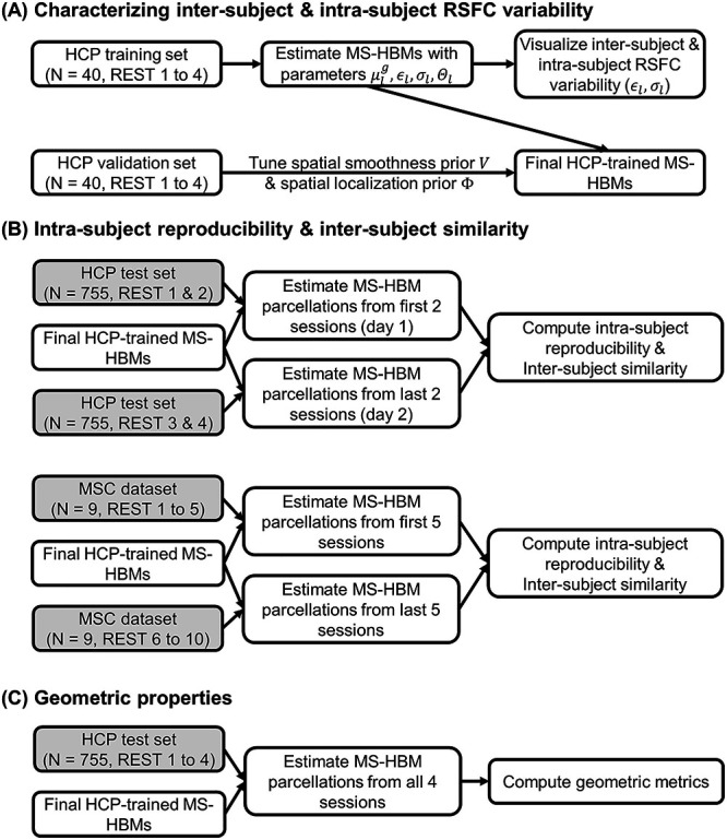
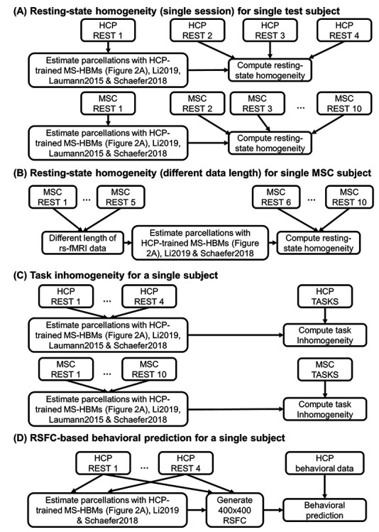
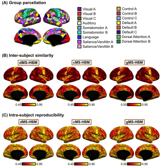
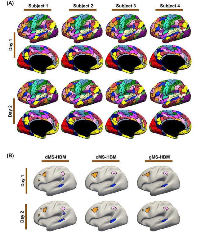
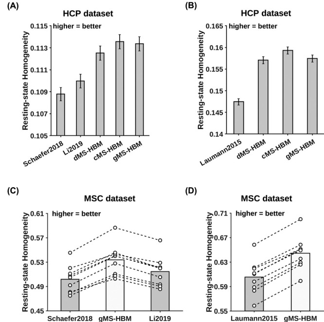
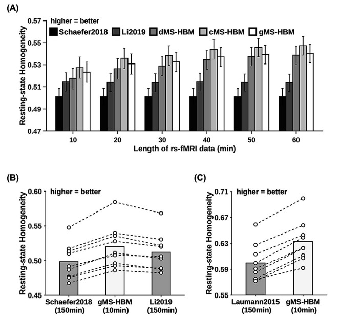
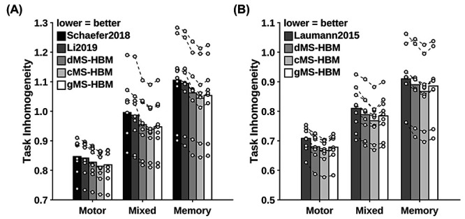
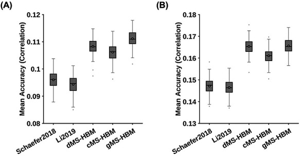
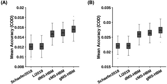
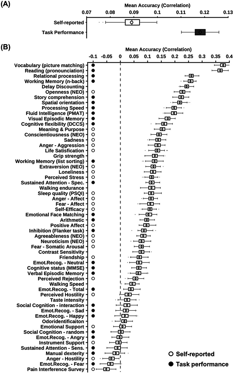
Resting-state functional magnetic resonance imaging (rs-fMRI) allows estimation of individual-specific cortical parcellations. We have previously developed a multi-session hierarchical Bayesian model (MS-HBM) for estimating high-quality individual-specific network-level parcellations. Here, we extend the model to estimate individual-specific areal-level parcellations. While network-level parcellations comprise spatially distributed networks spanning the cortex, the consensus is that areal-level parcels should be spatially localized, that is, should not span multiple lobes. There is disagreement about whether areal-level parcels should be strictly contiguous or comprise multiple noncontiguous components; therefore, we considered three areal-level MS-HBM variants spanning these range of possibilities. Individual-specific MS-HBM parcellations estimated using 10 min of data generalized better than other approaches using 150 min of data to out-of-sample rs-fMRI and task-fMRI from the same individuals. Resting-state functional connectivity derived from MS-HBM parcellations also achieved the best behavioral prediction performance. Among the three MS-HBM variants, the strictly contiguous MS-HBM exhibited the best resting-state homogeneity and most uniform within-parcel task activation. In terms of behavioral prediction, the gradient-infused MS-HBM was numerically the best, but differences among MS-HBM variants were not statistically significant. Overall, these results suggest that areal-level MS-HBMs can capture behaviorally meaningful individual-specific parcellation features beyond group-level parcellations. Multi-resolution trained models and parcellations are publicly available (https://github.com/ThomasYeoLab/CBIG/tree/master/stable_projects/brain_parcellation/Kong2022_ArealMSHBM).

Keywords: behavioral prediction; brain parcellation; difference; individual; resting-state functional connectivity.

Figure 1

(A) MS-HBM of individual-specific areal-level parcellations. denote the RSFC profile at brain location of subject during rs-fMRI session . The shaded circle indicates that are the only observed variables. The goal is to estimate the parcel label for subject at location given RSFC profiles from all sessions. is the group-level RSFC profile of parcel . is the subject-specific RSFC profile of parcel . A large indicates small inter-subject RSFC variability, that is, the group-level and subject-specific RSFC profiles are very similar. is the subject-specific RSFC profile of parcel during session . A large indicates small intra-subject RSFC variability, that is, the subject-level and session-level RSFC profiles are very similar. captures inter-region RSFC variability. A large indicates small inter-region variability, that is, two locations from the same parcel exhibit very similar RSFC profiles. Finally, captures inter-subject variability in the spatial distribution of parcels, smoothness prior encourages parcel labels to be spatially smooth, and the spatial localization prior ensures each parcel is spatially localized. The spatial localization prior is the crucial difference from the original network-level MS-HBM (Kong et al. 2019). (B) Illustration of three different spatial localization priors. Individual-specific parcellations of the same HCP participant were estimated using dMS-HBM, cMS-HBM, and gMS-HBM. Four parcels depicted in pink, red, blue, and yellow are shown here. All four parcels estimated by dMS-HBM were spatially close together but contained two separate components. All four parcels estimated by cMS-HBM were spatially contiguous. Three parcels (pink, red, and yellow) estimated by gMS-HBM were spatially contiguous, while the blue parcel contained two separate components.

Figure 2

Flowcharts of analyses characterizing MS-HBMs. (A) Training MS-HBMs with HCP training and validation sets, as well as characterizing inter-subject and intra-subject RSFC variability. (B) Exploring intra-subject reproducibility and inter-subject similarity of MS-HBM parcellations using HCP test set and MSC dataset. (C) Characterizing geometric properties of MS-HBM parcellations using HCP test set. Shaded boxes (HCP test set and MSC dataset) were solely used for evaluation and not used at all for training or tuning the MS-HBM models.

Figure 3

Flowcharts of comparisons with other algorithms. (A) Comparing out-of-sample resting-state homogeneity across different parcellation approaches applied to a single rs-fMRI session. (B) Comparing out-of-sample resting-state homogeneity across different parcellation approaches applied to different lengths of rs-fMRI data. (C) Comparing task inhomogeneity across different approaches. (D) Comparing RSFC-based behavioral prediction accuracies across different approaches. Across all analyses, MS-HBM parcellations were estimated using the trained models from Figure 2A. We remind the reader that the trained MS-HBMs were estimated using the HCP training and validation sets (Fig. 2A), which did not overlap with the HCP test set utilized in the current set of analyses. In the case of analyses (A) and (B), only a portion of rs-fMRI data was used to estimate the parcellations. The remaining rs-fMRI data were used to compute out-of-sample resting-state homogeneity. For analyses (C) and (D), all available rs-fMRI data were used to estimate the parcellations. Finally, we note that the local gradient approach (Laumann2015) does not yield a fixed number of parcels. Thus, the number of parcels is variable within an individual with different lengths of rs-fMRI data, so Laumann2015 was not considered for analysis B. Similarly, the number of parcels is different across participants, so the sizes of the RSFC matrices are different across participants. Therefore, Laumann2015 was also not utilized for analysis D.

Figure 4

Individual-specific MS-HBM parcellations show high within-subject reproducibility and low across-subject similarity in the HCP test set. (A) The 400-region Schaefer2018 group-level parcellation. (B) Inter-Subject spatial similarity for different parcels. (C) Intra-Subject reproducibility for different parcels. Yellow color indicates higher overlap. Red color indicates lower overlap. Individual-specific MS-HBM parcellations were generated by using day 1 (first two runs) and day 2 (last two runs) separately for each participant. Sensory-motor parcels exhibited higher intra-subject reproducibility and inter-subject similarity than association parcels.

Figure 5

MS-HBM parcellations exhibit individual-specific features that are replicable across sessions. (A) The 400-region individual-specific gMS-HBM parcellations were estimated using rs-fMRI data from day 1 and day 2 separately for each HCP test participant. Right hemisphere parcellations are shown in Supplementary Figure S2. See Supplementary Figures S3 and S4 for dMS-HBM and cMS-HBM. (B) Replicable individual-specific parcellation features in a single HCP test participant for dMS-HBM, cMS-HBM, and gMS-HBM.

Figure 6

MS-HBM parcellations achieved better out-of-sample resting-state homogeneity than other approaches. (A) The 400-region individual-specific parcellations were estimated using a single rs-fMRI session and resting-state homogeneity was computed on the remaining sessions for each HCP test participant. Error bars correspond to standard errors. (B) Same as (A) except that Laumann2015 allowed different number of parcels across participants, so we matched the number of MS-HBM parcels to Laumann2015 for each participant. Therefore, the numbers for (A) and (B) were not comparable. (C) The 400-region individual-specific parcellations were estimated using a single rs-fMRI session and resting-state homogeneity was computed on the remaining sessions for each MSC participant. Each circle represents one MSC participant. Dash lines connect the same participants. (D) Same as (C) except that Laumann2015 allowed different number of parcels across participants, so we matched the number of MS-HBM parcels to Laumann2015 for each participant. Results for dMS-HBM and cMS-HBM in the MSC dataset are shown in Supplementary Figure S9.

Figure 7

MS-HBM parcellations achieved better out-of-sample resting-state homogeneity with less amount of data. (A) The 400-region individual-specific parcellations were estimated using different lengths of rs-fMRI data for each MSC participant. Resting-state homogeneity was evaluated using leave-out sessions. Error bars correspond to standard errors. (B) The 400-region individual-specific parcellations were estimated for each MSC participant using 10 min of rs-fMRI data for gMS-HBM and 150 min of rs-fMRI data for Li2019. Each circle represents one MSC participant. Dash lines connect the same participants. (C) Same as (B) except that Laumann2015 yielded different number of parcels for each participant, so we matched the number of MS-HBM parcels accordingly for each participant. Results for dMS-HBM and cMS-HBM are shown in Supplementary Figure S10.

Figure 8

MS-HBM parcellations achieved better task inhomogeneity in the MSC dataset. (A) The 400-region individual-specific parcellations were estimated using all resting-state fMRI sessions. Task inhomogeneity was evaluated using task fMRI. Task inhomogeneity was then defined as the SD of task activation within each parcel and then averaged across all parcels and contrasts within each behavioral domain. Lower value indicates better task inhomogeneity. Each circle represents one MSC participant. Dash lines connect the same participants. (B) Same as (A) except that Laumann2015 yielded different number of parcels for each participant, so we matched the number of MS-HBM parcels accordingly for each participant. HCP results are shown in Supplementary Figure S11.

Figure 9

MS-HBM achieves the best behavioral prediction performance as measured by Pearson’s correlation. (A) Average prediction accuracies (Pearson’s correlation) of all 58 behavioral measures. Boxplots utilized default Matlab parameters, that is, box shows median and interquartile range (IQR). Whiskers indicate 1.5 IQR (not SD). Circle indicates mean. dMS-HBM, cMS-HBM, and gMS-HBM achieved average prediction accuracies of r = 0.1083 ± 0.0031 (mean ± SD), 0.1062 ± 0.0031, and 0.1111 ± 0.0031, respectively. On the other hand, Schaefer2018 and Li2019 achieved average prediction accuracies of r = 0.0960 ± 0.0031 and 0.0944 ± 0.0031, respectively. (B) Average prediction accuracies (Pearson’s correlation) of 36 behavioral measures with accuracies (Pearson’s correlation) higher than 0.1 for at least one approach (“36 behaviors > 0.1”). dMS-HBM, cMS-HBM, and gMS-HBM achieved average prediction accuracies of r = 0.1630 ± 0.0034 (mean ± SD), 0.1590 ± 0.0035, and 0.1656 ± 0.0036, respectively. On the other hand, Schaefer2018 and Li2019 achieved average prediction accuracies of r = 0.1442 ± 0.0036 and 0.1444 ± 0.0035, respectively.

Figure 10

MS-HBM achieves the best behavioral prediction performance as measured by COD. (A) Average prediction accuracies (COD) of all 58 behavioral measures. Boxplots utilized default Matlab parameters, that is, box shows median and interquartile range (IQR). Whiskers indicate 1.5 IQR (not SD). Circle indicates mean. dMS-HBM, cMS-HBM, and gMS-HBM achieved average prediction accuracies (COD) = 0.0147 ± 0.0009 (mean ± SD), 0.0149 ± 0.0009, and 0.0156 ± 0.0010, respectively. On the other hand, Schaefer2018 and Li2019 achieved average prediction accuracies (COD) = 0.0120 ± 0.0009 and 0.0121 ± 0.0009, respectively. (B) Average prediction accuracies (COD) of 36 behavioral measures with accuracies (Pearson’s correlation) greater than 0.1 for at least one approach (“36 behaviors > 0.1”). dMS-HBM, cMS-HBM, and gMS-HBM achieved average prediction accuracies (COD) = 0.0252 ± 0.0014 (mean ± SD), 0.0257 ± 0.0014, and 0.0266 ± 0.0014, respectively. On the other hand, Schaefer2018 and Li2019 achieved average prediction accuracies (COD) = 0.0212 ± 0.0014 and 0.0213 ± 0.0014, respectively.

Figure 11

Task performance measures were predicted better than self-reported measures across different parcellation approaches. Prediction accuracies were averaged across all parcellation approaches (three MS-HBM variants, Schaefer2018, and Li2019). (A) Prediction accuracies averaged across HCP task-performance measures (gray) and HCP self-reported measures (white). (B) Behavioral measures were ordered based on average prediction accuracies. Gray color indicates task performance measures. White color indicates self-reported measures. Boxplots utilized default Matlab parameters, that is, box shows median and interquartile range (IQR). Whiskers indicate 1.5 IQR (not SD). Circle indicates mean. Designation of behavioral measures into “self-reported” and “task-performance” measures followed previous studies (Liégeois et al. 2019; Li et al. 2019a).

References

1. Amunts K, Zilles K. 2015. Architectonic mapping of the human brain beyond Brodmann. Neuron. 88:1086–1107. - PubMed
1. Anderson KM, Collins MA, Kong R, Fang K, Li J, He T, Chekroud AM, Yeo BTT, Holmes AJ. 2020. Convergent molecular, cellular, and cortical neuroimaging signatures of major depressive disorder. PNAS. 117:25138–25149. - PMC - PubMed
1. Arcaro MJ, Schade PF, Vincent JL, Ponce CR, Livingstone MS. 2017. Seeing faces is necessary for face-domain formation. Nat Neurosci. 20:1404–1412. - PMC - PubMed
1. Arslan S, Parisot S, Rueckert D. 2015. Joint spectral decomposition for the parcellation of the human cerebral cortex using resting-state fMRI. In: Ourselin S, Alexander DC, Westin C-F, Cardoso MJ, editors. Information processing in medical imaging. Springer International Publishing: Cham, pp. 85–97. - PubMed
1. Barch DM, Burgess GC, Harms MP, Petersen SE, Schlaggar BL, Corbetta M, Glasser MF, Curtiss S, Dixit S, Feldt C, et al. 2013. Function in the human connectome: task-fMRI and individual differences in behavior. Neuroimage. 80:169–189. - PMC - PubMed
Publication types