. 2021 May;593(7860):558-563.
doi: 10.1038/s41586-021-03514-2. Epub 2021 May 5.

Fast odour dynamics are encoded in the olfactory system and guide behaviour

Affiliations

Fast odour dynamics are encoded in the olfactory system and guide behaviour

Tobias Ackels et al. Nature. 2021 May.

Abstract

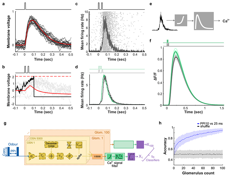
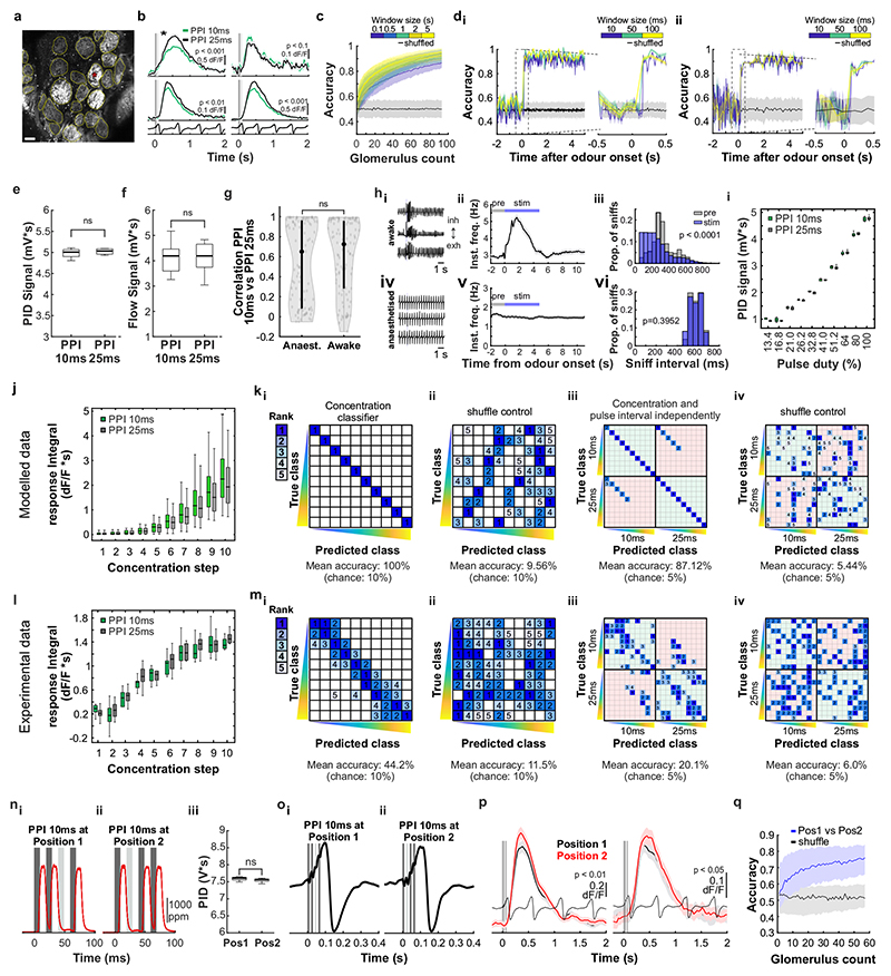
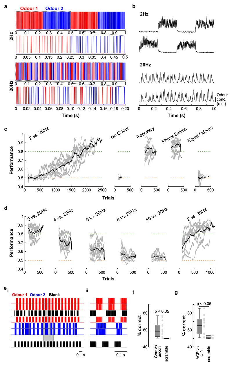
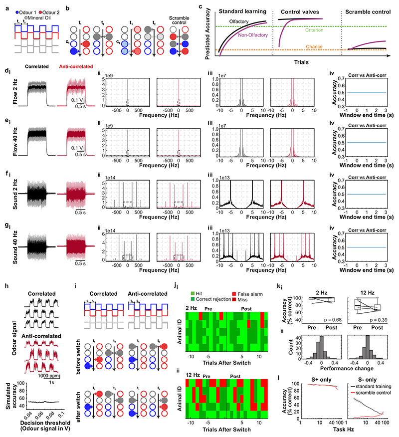
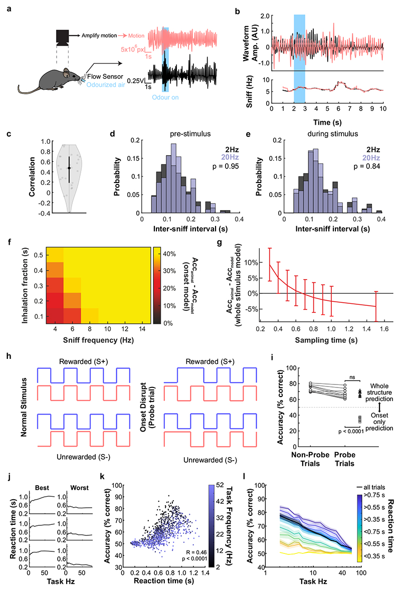
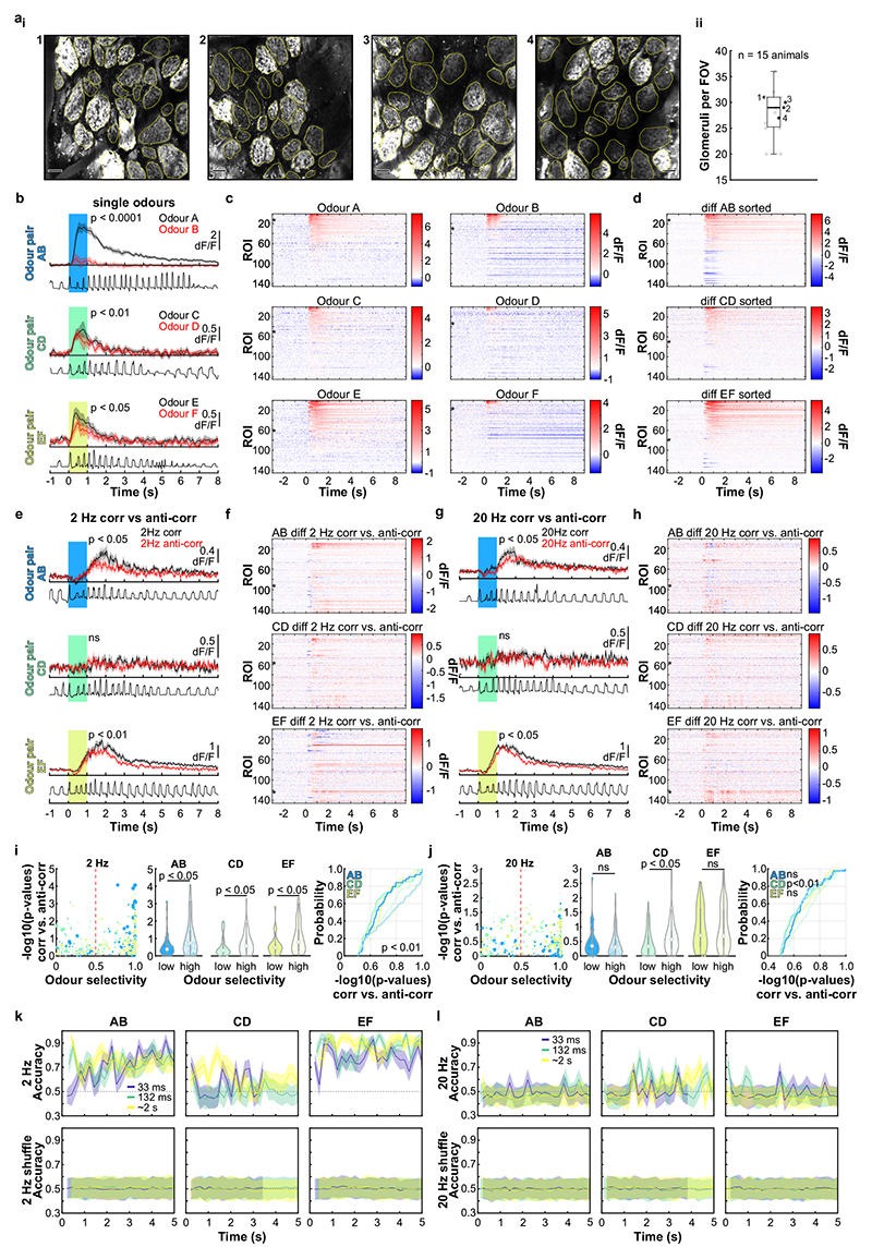
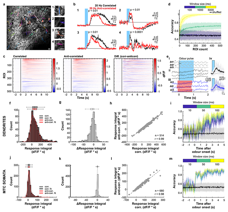
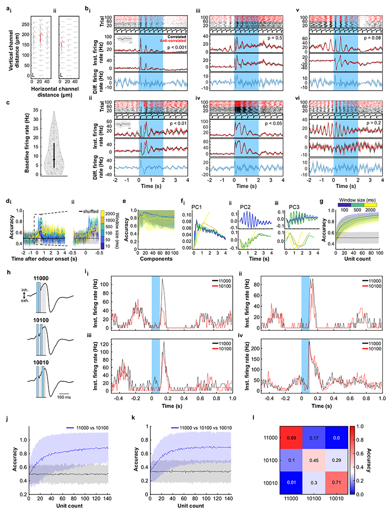
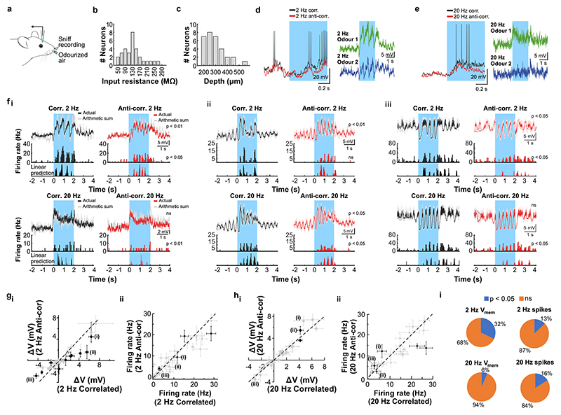
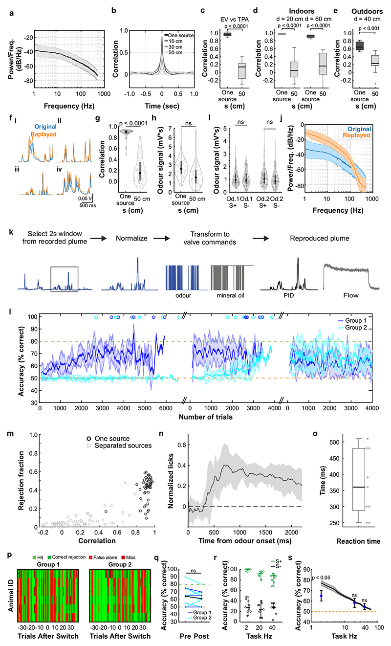
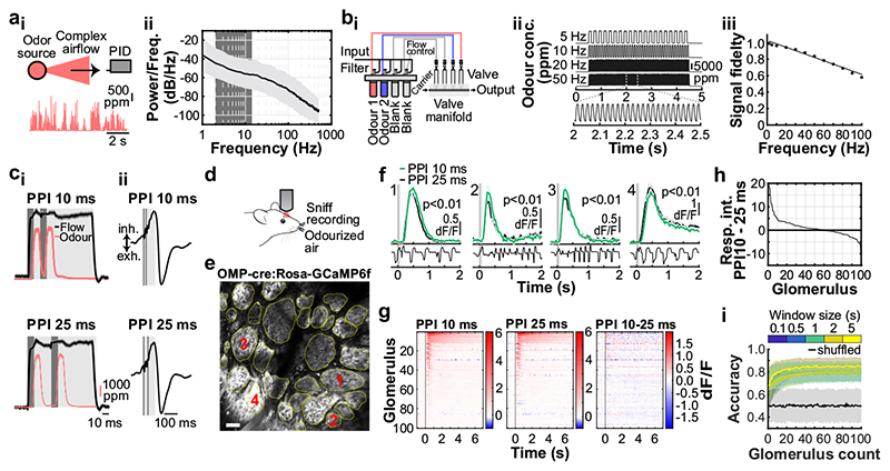
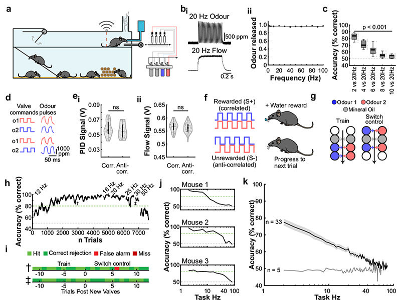
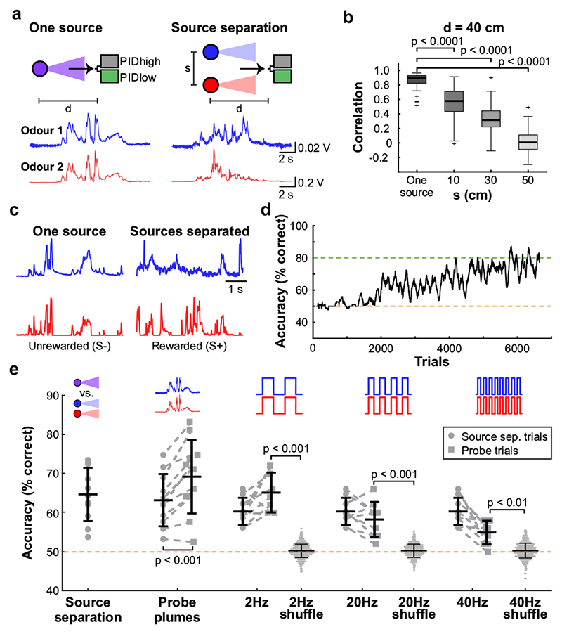
Odours are transported in turbulent plumes, which result in rapid concentration fluctuations1,2 that contain rich information about the olfactory scenery, such as the composition and location of an odour source2-4. However, it is unclear whether the mammalian olfactory system can use the underlying temporal structure to extract information about the environment. Here we show that ten-millisecond odour pulse patterns produce distinct responses in olfactory receptor neurons. In operant conditioning experiments, mice discriminated temporal correlations of rapidly fluctuating odours at frequencies of up to 40 Hz. In imaging and electrophysiological recordings, such correlation information could be readily extracted from the activity of mitral and tufted cells-the output neurons of the olfactory bulb. Furthermore, temporal correlation of odour concentrations5 reliably predicted whether odorants emerged from the same or different sources in naturalistic environments with complex airflow. Experiments in which mice were trained on such tasks and probed using synthetic correlated stimuli at different frequencies suggest that mice can use the temporal structure of odours to extract information about space. Thus, the mammalian olfactory system has access to unexpectedly fast temporal features in odour stimuli. This endows animals with the capacity to overcome key behavioural challenges such as odour source separation5, figure-ground segregation6 and odour localization7 by extracting information about space from temporal odour dynamics.


Conflict of interest statement

The authors declare no competing financial interests.

Figures

Extended Data Fig. 1
Extended Data Fig. 1. Distinguishing fast odour stimuli with slow OSNs.
a, Membrane voltage relative to baseline of a single model OSN in response to a 10 ms odour pulse. Black traces are individual trials; red trace is average over 20 trials. OSN spike threshold has been set high enough to prevent spiking to illustrate the subthreshold voltage time course. b, Membrane voltages (grey traces) of ten OSNs from a population of 5000 in response to a paired odour pulse with pulse width 10 ms and PPI of 25 ms. The voltage time course for one example OSN is in black. Several OSNs reach the OSN spike threshold (dashed red line) and are temporarily reset to the refractory voltage of -1. The population average membrane voltage (red) reveals membrane charging in response to odour stimulation and the subsequent discharging and refractory period. c, Raster showing the spike times (dots) of the full population from b and the corresponding mean firing rate (trace) estimated in 1 ms bins. d, Mean firing rates computed over 20 trials in response to paired odour pulses of width 10 ms and PPIs of 10 ms (green) and 25 ms (black). e, Model calcium signals are produced by squaring the instantaneous mean firing rate and filtering the result with a calcium imaging kernel. f, Model calcium responses to the paired odour stimulus with a PPI of 10 ms (green) and 25 ms (black). Thin traces are single trials, thick traces are averages over 15 trials. g, Schematic of the OSN model. Variables in dashed bounding boxes are changed for each glomerulus (see Methods). h, Linear classifier analysis over an increasing subset size of glomeruli (1-100; plotted is mean ± SD, 256 repeats for random subsets of n glomeruli generating 256 unshuffled and 256 shuffled accuracies).
Extended Data Fig. 2
Extended Data Fig. 2. Sub-sniff odour information in the olfactory bulb input layer.
a, GCaMP6f fluorescence recorded in olfactory bulb glomeruli in an anaesthetised OMP-cre:Rosa-GCaMP6f mouse (maximum projection of 8200 frames, glomerulus marked with red asterisk corresponds to first example trace shown in b). Scale bar: 50 μm. b, Example calcium traces in response to 10 and 25 ms PPI odour stimuli (mean of 50 trials ± SEM). Bottom: Example respiration traces. P-values derived from unpaired two-sided t-tests comparing responses of individual trials integrated over 2 s windows to paired odour pulse stimulation. c, Classifier accuracy over an increasing number of glomeruli when a linear classifier was trained on several response windows (colour-coded black: shuffle control) to PPI 10 vs. 25 ms stimuli (mean ± SD of up to 93 glomeruli from 4 individual animals; 500 repetitions). di, Classifier accuracy when trained on all glomeruli in response to PPI 10 vs. 25 ms stimuli recorded in anaesthetised animals (n = 93 glomeruli, mean ± SD from 4 individual animals) with a sliding window of different durations (colour-coded; black: shuffle control; 100 repetitions) starting at 2 s before odour onset (left) and time period between -0.5 and 0.5 s from odour onset shown at higher magnification (right). dii, Same as di for awake animals (n = 100 glomeruli, mean ± SD from 5 individual animals). e, Odour and f, flow signal integrated over 2 s for PPI 10 ms and PPI 25 ms stimuli (10 repeats each, odour: p = 0.1841, flow: p = 0.1786, unpaired two-sided t-test). g, Correlation coefficients of glomerular calcium responses to PPI 10 vs. 25 ms in anaesthetised (n = 93 glomeruli from 4 individual animals) and awake (n = 100 glomeruli from 5 individual animals) mice (p = 0.3187, unpaired two-sided t-test, measured as in Fig. 1 from OMP-Cre:Rosa-GCaMP6f mice). Violin plots show the median as a black dot and the first and third quartile by the bounds of the black bar. hi, Example respiration traces recorded using a flow sensor from awake mice. Inhalation goes in the upwards, exhalation in the downwards direction. hii, Average instantaneous sniff frequency from one example animal plotted as a function of time (n = 24 trials, mean ± SEM). The odour stimulus consisted of two 10 ms long odour pulses either 10 or 25 ms apart (see Fig. 1c). hiii, Distribution of sniff intervals during a 2 s window before (grey) and a 5 s window after (blue) odour stimulus onset (p = 1.02e-189, two-sample Kolmogorov-Smirnov test). hiv-vi, Same but for the anaesthetised condition (p = 0.3952, two-sample Kolmogorov-Smirnov test). i, Mean odour signal for PPI 10 and 25 ms for 10 increasing concentration steps defined by modulating valve pulse duty (see Methods and Supplementary Methods Fig. 1). There were no significant differences in odour concentration between both stimuli (unpaired two-sided t-tests). j, Modelled response integrals to PPI 10 vs. 25 ms stimulations over a 10-fold concentration range pooled over all 20 trials and 100 glomeruli (see Methods). Box plots show median and extend from the 25th to 75th percentiles, whiskers extend to the 5th and 95th percentiles. ki, Confusion matrix of support vector machine (SVM)-based classification results of modelled glomerular signals in response to a range of 10 odour concentrations ranked and colour-coded (n = 100 glomeruli). kii, Shuffle control with labels assigned randomly. kiii, Confusion matrix showing the ranked and colour-coded results of glomerular responses independently classified for 10 ms vs. 25 ms PPI and across the range of 10 odour concentrations. kiv, Shuffle control for kiii with labels assigned randomly. l, Same as j but 2 s response integrals are derived from Ca2+ imaging data (10 repeats for each concentration). m, Same as k for Ca2+ imaging data (n = 57 glomeruli, from 2 individual animals, 10 repeats for each concentration). Note that 10 ms PPI could be reliably distinguished from 25 ms PPI with only few instances where a response to e.g. a 10 ms PPI stimulus was misclassified as 25 ms or vice versa (compare light red quadrants to light green quadrants). n, Shifting the position of 10 ms PPI within a single inhalation. ni, PPI 10 ms at Position 1 or nii, at Position 2 of three 10 ms odour pulses. Odour pulses as recorded with a PID shown in red, valve commands are shown in dark grey. Light grey area shows additional compensatory blank valve command to keep the flow profile indistinguishable between stimuli. niii, Total odour concentration was independent of the pulse profile (10 repeats, p = 0.57, unpaired two-sided t-test). o, Both the 10 ms PPI at Position 1 (oi) and at Position 2 (oii) are presented during the inhalation phase (respiration shown in black, inhalation upwards, exhalation downwards). p, Example calcium traces in response to 10 ms PPI at Position 1 (black) and Position 2 (red), shown is the mean of 10 trials ± SEM. P-values derived from unpaired t-tests comparing 2 s integrated responses of individual trials to odour pulses. q, Classifier accuracy over increasing number of glomeruli when a linear classifier was trained on the 2 s response to PPI 10 ms at Position 1 vs. Position 2 (mean ± SD of up to 57 glomeruli, from 2 individual animals, 500 repetitions; blue: PPI 10 ms at Position 1 vs. Position 2, black: shuffle control). Boxes in e,f,niii indicate 25th–75th percentiles, thick line is median, whiskers are most extreme data points not considered outliers (see Methods).
Extended Data Fig. 3
Extended Data Fig. 3. Frequency discrimination experiments.
a, Frequency discrimination stimuli are produced by alternating presentation of two odours to generate a desired odour change frequency. During odour delivery, valves are not held open but rather randomly opened and closed over time to produce slight variation in odour amplitude for each pulse. This means that odour concentration cannot be used as a cue to learn the task and odour switching frequency is the primary stimulus signal. Furthermore, valve clicking is randomised to minimize any acoustic cues. b, Replacing one odour channel with blank, un-odourised air and recording the frequency stimuli with a PID reveals that the desired odour pulse frequency is being produced. c, Mice readily learn to discriminate 2 vs. 20 Hz pulse frequency stimuli in a go/no-go task. Replacing the odours with blank channels results in chance-level performance (No odour), which recovers when odours are replaced (Recovery) showing that mice were likely discriminating the odour switching frequency rather than any extraneous cues such as valve noise. The order of odour presentation in the stimuli had no effect on behaviour as when it was shifted (Phase switch) no decrease in performance was observed. Additionally, performance was dependent on the alternation between different odours as when the experiment was repeated with the same odours in each channel (Equal odours) performance was at chance level. d, To determine the perceptual limit of frequency discrimination, the floor frequency used in the task over successive experiments was increased such that the difference in frequency between the stimuli progressively narrowed. Overall performance decreased as the difference in frequency grew smaller, reaching near-chance level with a frequency difference of 10 Hz (10 vs. 20 Hz). Switching back to the original discrimination (2 vs. 20 Hz) recovered performance quickly, showing that the drop in discrimination ability was truly due to the frequency difference rather than general deterioration of performance over time. e, Example uncorrelated stimuli. Combinations of odour 1 (red) and odour 2 (blue) valves are opened with temporal offsets and randomised pulse timing resulting in a correlation of 0 (see Methods). Blank (black) valves are used to keep total airflow constant throughout the stimulus. eii, Higher magnification of the area in ei marked in grey. f, Animals show similar average accuracy as shown in Fig. 2k when probed to discriminate correlated from uncorrelated odour pulses at 10 Hz (n = 19 mice, mean ± SEM of average accuracy = 0.6506 ± 0.0016; after scrambling stimulus identity: 0.4997 ± 0.0032; p = 0.0175, unpaired two-sided t-test). g, Animals show similar average accuracy when discriminating the correlation structure of a different odour pair (Acetophenone vs. Cineol) at 10 Hz (n = 19 mice, mean ± SEM of average accuracy = 0.6558 ± 0.0026; after scrambling stimulus identity: 0.5165 ± 0.0048; p = 0.0129, unpaired two-sided t-test). Grey dots mark average performance of individual animals. Boxes in f,g indicate 25th - 75th percentiles, thick line is median, whiskers are most extreme data points not considered outliers (see Methods).
Extended Data Fig. 4
Extended Data Fig. 4. AutonoMouse stimulus and experimental design.
a, Detailed schematic of stimulus production; odour presentation (Odour 1: blue, Odour 2: red) is always offset by clean air (Mineral Oil: grey) valves at the same flow levels, to ensure that total flow during the stimulus is constant. b, Schematic of the use of valve subsets to produce the desired stimulus. t1 and t2 represent valve openings at the corresponding time points shown in a. c1 (b, left) and c2 (b, middle) represent two possible configurations that could be used to produce the same resulting stimulus at the two time points. Opacity in the colours represents total concentration contribution to the resulting stimulus at the time point. For example, to produce the dual odour pulse at t1, configuration c1 can be used where odour 1 (blue) is delivered from one valve and odour 2 (red) from another valve. During t2 two valves contribute clean air. Alternatively, configuration c2 can be used in which during t1 odour 1 (blue) is generated by 50% opening of two valves, with odour 2 (red) produced by 70% / 30% opening of two other valves respectively. (b, right) Scramble control: valve maps (represented by arrow colour) are maintained compared to the training condition but odour vial positions are scrambled resulting in odour stimuli uninformative about reward association whilst maintaining any non-odour cue such as putative sound or flow contributions. c, Predicted accuracy for animals in the case that they use solely olfactory temporal correlations (black) and in the case that they use extraneous non-olfactory cues or non-intended olfactory cues (e.g. contaminations, clicking noises) (violet). Note that when switching stimulus preparations to a new set of valves (as in Fig. 2i and below in i-k), such non-intended cues would not provide any information about stimulus-reward association, thus animals’ accuracies would transiently drop back to chance. di, Average flow recordings (mean ± SD) of 2 Hz correlated (black, n = 75) and anti-correlated (red, n = 70) trials taken from the AutonoMouse odour port. dii, Fourier transform of the flow plots from di, showing the power of the signal over a range of 1 kHz. diii A zoom in over the range of 10 Hz indicated by the dotted box in dii. div, Mean accuracy of a series of linear classifiers trained on an increasing window of the integrated signal starting from 1 s before trial shown in di. Classifiers were tested on two withheld trials, one correlated and one anti-correlated, and repeated 100 times. e, Same as d but for 40 Hz trials (n = 69 correlated and n = 72 anti-correlated). fi, Average audio recording trace (mean ± SD) of 2 Hz stimuli using a microphone placed in close proximity to the AutonoMouse odour port. fii, fiii, Fourier transforms of the audio signal from fi. Note, whilst there are notable peaks at specific frequencies, these are present in both correlated and anti-correlated trials. fiv, Accuracy of a series of linear classifiers as shown in d but using the modulus of the audio signal. g, Same as f but for 40 Hz trials. Note, whilst the sound profile and the Fourier transforms are different between 2 and 40 Hz, there is no difference detectable between correlated and anti-correlated trials. h, Example traces of odour signal (ethyl butyrate, isoamyl acetate, PID recorded) during correlated (top) and anti-correlated trials (middle). Simulated maximum accuracy based on differences in mean odour signal (bottom). Simulated accuracy was calculated as the fraction of trials correctly identified as correlated / anti-correlated based on a decision threshold set at some level between the minimum and maximum mean signal. Simulated accuracy was calculated for multiple decision thresholds, increasing the decision threshold from minimum odour signal to maximum odour signal in steps of 1/5000th of the range between minimum and maximum. i, Detailed schematic of correlated (top left) and anti-correlated (top right) stimulus production before (middle) and after (bottom) switching valves. For the switch control, a set of previously unused odour valves is introduced to rule out potential bias towards a specific valve combination when performing the odour correlation discrimination task. j, Trial map of 5 representative animals during 2 Hz (ji) and 12 Hz (jii) correlation discrimination tasks before and after introduction of control valves (n = 12 trials pre-, n = 12 trials post-new valve introduction, new valve introduction indicated by black vertical dotted line. Each row corresponds to an animal, each column within the row represents a trial. Light green: hit, dark green: correct rejection, light red: false alarm, dark red: miss. ki, Boxplots of mean accuracy for animals (n = 5 mice) pre- and post-control for 2 Hz (left) and 12 Hz (right). Box indicates 25th – 75th percentiles, thick line is median, whiskers are most extreme data points not considered outliers, see Methods. P-values derived from unpaired t-tests. k", Summary histograms of performance change for all animals during all “valve switch” control tests (see Methods) indicating that discrimination accuracy was based on intended olfactory cues. The five animals showing highest performance before the valve switch/bottle change (and thus the largest potential to drop in performance) were analysed. l, Discrimination accuracy (n = 33 animals, mean ± SEM) for rewarded S+ (left) and unrewarded S- (right) trials when odours were presented using standard training valve configurations (black) and scrambled valve identity (red), data from Fig. 2k. Note that frequencies >40 Hz were presented predominantly in the last block of the training schedule and reduced licking in the control group (decreased S+ performance and increased S- performance) might be due to decreased motivation at that point.
Extended Data Fig. 5
Extended Data Fig. 5. Respiration recordings, stimulus onset model and reaction time for correlation discrimination experiments.
a, An overhead camera was used to image a head-fixed mouse during a sequence of odour presentations. Simultaneously, a flow sensor was placed close to one nostril to monitor respiration to establish the validity of motion imaging-based respiration recording. Phase-based motion amplification was used to magnify motion on the animal’s flank to capture body movements associated with respiration. Right: example for simultaneous respiration measurement with motion imaging (red) and flow sensor (black; see Methods and Supplementary Video 2). b, Three further example trials with respiration rate extracted from motion imaging (red) and simultaneous flow sensor recording (black). Below: instantaneous sniff frequencies calculated from either sensor were tightly correlated. c, Correlation between respiration traces extracted from motion imaging and respiration captured by flow sensor (n = 26 trials, 10 s duration each). Violin plot shows the median as a black dot and the first and third quartile by the bounds of the black bar. d, Probability distributions of inter-sniff intervals for odour presentations (isoamyl acetate vs. ethyl butyrate, 2 Hz and 20 Hz) for freely moving animals in AutonoMouse before stimulus onset and e, during 2 s odour stimulation (n = 605 sniffs for 2 Hz and n = 668 for 20 Hz, two-sample Kolmogorov-Smirnov test). f, Heat map of accuracy difference between a model where animals rely on onset information only (see Methods) and actual animal accuracies across a range of sniff frequencies and inhalation fractions (n = 10 mice). No matter what assumed sniff frequency and inhalation frequency, the “onset model” deviates substantially from the accuracy measured in the behavioural experiments (panels h,i). g, Difference between a model where animals use the entire stimulus structure (see Methods) and actual behavioural accuracies across different stimulus sampling times (n = 10 repeats, mean ± SD). The “whole stimulus” model accurately describes animal behaviour indicating that mice base a decision about the correlation structure of a stimulus not predominantly on the onset. Note the different scales in f and g. h, Schematic of experimental stimulus in which the first stimulus pulse was disrupted when presented on “probe trials”. Top: normal stimulus design, bottom: “onset disrupt” stimuli in which the first pulse in a correlated stimulus is disrupted to be anti-correlated; and vice versa for an anti-correlated stimulus. i, Animals were trained on standard (non-probe) correlation discrimination stimuli (f = 10 Hz) but onset disrupt (probe) stimuli were presented randomly on probe trials with a 1/10 probability. Accuracy was only slightly degraded on probe trials (mean ± SD of accuracy for non-probe trials 75.8 ± 4.4%; for probe trials 67.8 ± 6.1%; p = 0.001, paired two-sided t-test, n = 9 mice) but did not drop below chance (p = 7.3e-06, paired t-test). Importantly, accuracy on probe trials was consistent with whole-structure prediction (70.3 ± 3.5%, p = 0.13, paired t-test of comparison to probe trials) and differed significantly from the accuracy of onset-only prediction (41.6 ± 1.5%; p = 1.02e-6, paired t-test of comparison to probe trials). j, Mean reaction time (time from stimulus onset to first lick in S+ trials) plotted as a function of stimulus pulse frequency for the three animals with the best (left) and the worst (right) global accuracy (mean accuracy across all trials). Better performing animals tend to increase their reaction time as stimulus pulse frequency increases. k, Scatter plot of mean accuracy vs. mean reaction time for each animal and stimulus pulse frequency condition (averaged over blocks of 100 trials). Points are colour-coded according to stimulus pulse frequency. Accuracy was significantly positively correlated to reaction time, suggesting that mice that sampled a greater portion of the stimulus made more accurate decisions about its correlation structure (Pearson correlation coefficient R = 0.49, p<1.1e-112). l, Accuracy (mean ± SEM) is plotted as in Fig. 2k, but only trial blocks with reaction times above or below a certain threshold (colour code) are included in the analysis. Where only longer reaction times are considered, global performance is higher than the case where only shorter reaction times are included, again suggesting that longer stimulus sampling improves discrimination of odour correlation structure across all stimulus pulse frequencies.
Extended Data Fig. 6
Extended Data Fig. 6. OSN imaging in response to correlated vs. anti-correlated odour stimulation.
a, Four example fields of view (FOV) recorded from the dorsal olfactory bulb of individual mice. aii, Number of individual glomeruli per FOV in all experimental mice (n = 15). The number of individually delineated glomeruli ranges from 20-36 with an average of 28 glomeruli per FOV. Labelled data points (1-4) correspond to FOVs shown in ai. Scale bars: 50 μm. Edges of the box are the 25th and 75th percentiles, the whiskers extend to the most extreme data points not considered as outliers, see Methods. b, Example glomerulus response from OMP-Cre:Rosa-GCaMP6f mice to presentation of individual odours plotted pairwise (AB, CD, EF; mean of 6 trials ± SEM). Stimulation period (1 s) is indicated by vertical bar (blue, green and yellow). Bottom: Typical example respiration trace. P-values derived from unpaired two-sided t-tests comparing 2 s integrated responses between paired odours. c, Averaged calcium transients from all glomeruli (n = 145 from 5 individual animals) in response to individual odours, plotted as colour maps sorted by response magnitude. d, Difference between glomerulus responses to individual odours plotted pairwise as colour maps. Glomeruli are sorted by average magnitude of response difference. e, Example glomerulus response to presentation of correlated vs. anti-correlated odour pairs fluctuating at 2 Hz (mean of 12 trials ± SEM). Bottom: typical example respiration trace. P-values derived from unpaired two-sided t-tests comparing 2 s integrated responses of individual trials to correlated and anti-correlated odour stimulation. f, Difference between glomerulus responses to 2 Hz correlated and anti-correlated odours as colour maps sorted as shown in d. g-h, Same as in e-f but for 20 Hz correlated vs. anti-correlated. Example glomerulus from b,e,g indicated with an asterisk in colour maps in c,d,f,h. i, Left: P-values derived from comparing trials of the summed 2 s response to correlated vs. anti-correlated odour stimulation at 2 Hz (unpaired two-sided t-tests) for three odour pairs (colour-coded) as a function of glomerulus selectivity to individual odours (n = 145 glomeruli). Selectivity is calculated as the difference between the absolute response to single odours scaled by the summed absolute response. A threshold is set at 0.5 defining glomeruli as low or high selective. Dot size represents magnitude of the summed response. Middle: Comparison of p-values between low and high selective glomeruli (p < 0.05, unpaired two-sided t-test). Violin plots show the median as a white dot and the first and third quartile by the bounds of the grey bar. Right: Cumulative distribution function of p-values for low and high selective glomeruli (p < 0.01 for all pairwise comparisons, two-sample Kolmogorov-Smirnov test). j, Same as i but for 20 Hz, (n = 145 glomeruli). k, Top row: Mean ± SD over 100 repetitions of classifier accuracy when trained on all responsive glomeruli (n = 145 available, from 5 individual animals, see Methods) to discriminate 2 Hz correlated vs. anti-correlated stimuli, trained separately for each of the three odour pairs and within sliding windows of different widths (colours); x-coordinates indicate latest extent of each window. Bottom row: same as top row but with labels shuffled as control. l, Same as k for 20 Hz correlated vs. anti-correlated odours. Some data points in k, l are absent because not all time points had responsive ROIs for every window size (see Methods).
Extended Data Fig. 7
Extended Data Fig. 7. Odour correlation structure is encoded in dendrites of olfactory bulb output neurons.
a, GCaMP6f fluorescence from mitral and tufted cells and their dendrites recorded in the dorsal portion of the olfactory bulb of a Tbet-cre:Rosa-GCaMP6f mouse (maximum projection of 8000 frames). Dendritic ROIs are superimposed in colour. Four dendritic segments (1-4) are shown in higher magnification, scale bars: 20 μm. b, Four example calcium traces extracted from dendritic segments shown in a that show differential response kinetics to correlated (black) and anti-correlated (red) stimulation (mean of 24 trials ± SEM, f = 20 Hz). In total, 24% of dendritic segments showed significantly different integral responses (0-5 s after odour onset, p < 0.01, unpaired two-sided t-test; 121/514) to the two stimuli. c, Average calcium transients as colour maps for correlated (left) anti-correlated (middle) and the difference between both odour stimulations (right) of all analysed dendritic segments (n = 514, from 6 individual animals). d, Classifier accuracy over an increasing number of dendritic ROIs trained on several response windows (colour-coded) to discriminate correlated vs. anti-correlated stimuli at 20 Hz (n = up to 514, mean ± SD from 6 individual animals, black: shuffle control). e, Method of aligning calcium traces to first inhalation after odour stimulus onset. ei, Representative respiration traces recorded using a flow sensor placed in front of the nostril contralateral to the imaging window. The first inhalation peaks were detected and the time (Δt) to the first inhalation after odour onset was calculated for each trial individually. eii, Representative calcium transients in response to a single odour presentation (here: 20 Hz correlated). eiii, Transients are shifted according to Δt. eiv, Individual calcium transients (faint colours, 24 trials) in response to 20 Hz correlated odour presentations with the average calcium signal (thick traces) superimposed. Top: before aligning to first inhalation after odour onset, bottom: after alignment. Blue bar represents the odour presentation phase (approximate for the aligned data). f, Distribution of odour response integrals from all recorded ROIs (n = 514) for correlated (grey) and anti-correlated (red) stimulation. Box indicates 25th – 75th percentiles, thick line is median, whiskers are most extreme data points not considered outliers, see Methods. g, Histogram of the difference between correlated and anti-correlated odour responses. Box plots as in f. h, Comparison of correlated and anti-correlated odour responses of all dendritic ROIs (f = 20 Hz, n = 514 dendrites). i, Classifier accuracy when trained on all dendritic ROIs recorded with a sliding window of different durations starting 2 seconds before odour onset (colour-coded, black: shuffle control, n = 514 from 6 individual animals; mean ± SD, 100 repetitions). j-m, same as f-i for projection neuron somata (f = 20 Hz, n = 680 cells; see Fig. 3).
Extended Data Fig. 8
Extended Data Fig. 8. Projection neurons unit recordings in response to correlated vs. anti-correlated stimulation and short odour pulse combinations.
a, Data from unit recordings as described in Fig. 3h-k. Average waveforms across all channels of two isolated units shown in bi,ii. Each waveform represents the average waveform for the unit on a specific channel. Red waveform indicates the channel with the largest average waveform for the unit. Scale bar in the bottom left represents 100 μV (vertically) and 1 ms (horizontally). b, Additional example single unit odour responses to correlated (black) and anti-correlated (red) stimuli shown as raster plot (top) and PSTH (mean of 64 trials for each condition ± SEM) of spike times before (second from top) and after baseline subtraction (second to bottom), and the differential PSTH of correlated and anti-correlated (bottom, blue). Average spike waveform shown as insets in bi,ii. Duration of odour presentation (2 s) is indicated in light blue. P-values are derived from a two-sided Mann-Whitney U test comparing the spike time distributions of correlated and anti-correlated trials during 4 s after odour onset. c, Average baseline firing rate for all units (n = 97 from 6 individual animals). Baseline firing rates were calculated from 4 s to 0 s before odour onset for each of the 1312 trials presented during all recordings. Violin plot shows the median as a black dot and the first and third quartile by the bounds of the black bar. di, Classifier accuracy when trained on all baseline-subtracted units in response to 20 Hz correlated vs. anti-corelated stimulation (n = 97 units, mean ± SD from 6 individual animals) with a sliding window of different durations (colour-coded; black: shuffle control; 100 repetitions) starting at 2 s before odour onset. Time along the x-axis represents the end time of the window. dii, Time period between -0.5 and 0.5 s from odour onset shown at higher magnification (n = 97 units, mean ± SD from 6 individual animals). e, To take the entire temporal structure of responses into account we performed a principal component analysis (PCA) on the temporal evolution of the firing rate responses (see Methods). Shown here is the accuracy for linear SVM classifiers (mean ± SD) trained on increasing numbers of principal components (PCs). Classifiers were trained on all but two trials (one correlated, one anti-correlated). Training and testing were repeated 1000 times. The colour code represents the same window sizes as defined in d. f, The first (fi), second (fii), and third (fiii) PCs found from PCA for different rolling window sizes (colour code as defined in d). In the second and third PCs, the windows have been split as to better compare the similarities in PCs for different window sizes. g, Average classifier accuracy of a set of classifiers trained on the PC weights of increasing number of units. Classifiers were trained on all but two trials (one correlated, one anti-correlated). The number of PCs used for each window was selected by the peak accuracies in e (colour-coded; n = up to 97 units from 6 individual animals; mean ± SD of 1000 classifier repetitions). h, Schematic of odour pulse stimuli timings in relation to the respiration cycle. Three combinations were presented, each trial 120 ms in length. For example, 11000 (top) consisted of a 40 ms odour pulse (light blue) followed by 80 ms of blank odourless air (grey); All trials were triggered at the onset of inhalation. i, PSTH from four example units (ii-iv) showing their average firing rate prior, during, and after odour presentation (light blue vertical bar). Responses are either to 11000 trial (black) or 10100 odour presentation (red). The instantaneous firing rate was calculated by summing the number of detected spikes in 10 ms windows and multiplying the value by 100 to get Hz. j, Accuracy of linear classifiers as a function of the number of units available for training/testing (mean ± SD of n = up to 145 units from 8 individual anaesthetised animals). Each classifier is trained on the summed spike count of the available units in a window of 500 ms starting at odour onset. The classifiers were trained on all but two trials, one 11000 and one 10100 trial and the number of repeats between animals varied between 11 and 30. To account for this and to minimise the variability of the training set, trial number was bootstrapped to 1000 repeats. This was achieved by randomly selecting a repetition for each unit independently. The test set was isolated from the responses prior to bootstrapping and thus was not seen by the classifier until it was tested on it. Each classification was repeated 500 times with a different selection of units, and a different test set. The shuffled control (black) was accomplished by shuffling the training labels during each iteration of the classifier without shuffling test labels. k, Same as in j but classifying all three odour pulse combinations shown in h. l, Confusion matrix showing the fractions that each trial type was classified as (n = 145 units from 8 individual animals). True labels are shown on the x-axis and labels predicted by the classifier on the y-axis. Accuracies correspond to maximum unit count shown in c and d. The classifiers can readily separate between trials containing a single 40 ms odour pulse. Accuracy is lower when distinguishing between an intermission of 20 or 40 ms but remains above chance (chance = 0.33).
Extended Data Fig. 9
Extended Data Fig. 9. Whole cell recordings of projection neurons in response to correlated vs. anti-correlated odour stimulation.
a, Schematic of the whole-cell patch clamp recording approach. b, Distribution of input resistance and c, recording depth as measured from all recorded projection neurons (n = 31). d, Left: Example recording from single cells with consecutive presentations of correlated (black) and anti-correlated (red) odour stimulus at 2 Hz. Duration of odour presentation (2 s) is indicated in light blue. Right: Baseline-subtracted and spike-clipped subthreshold voltage response from a single cell to odour 1 (green) and odour 2 (blue) for 2 Hz. e, the same as d but for 20 Hz odour stimulation. f, Voltage response from three example cells for correlated (black) and anti-correlated (red) odour stimulus for 2 Hz (top) and 20 Hz (bottom). The cell shown in fi corresponds to the cell shown in d and e. The grey overlaid traces correspond to the arithmetic sum estimated from the response to individual odours. Bottom: Linear prediction histogram calculated by thresholding the arithmetic sum of the subthreshold responses to the individual odours. Differences here suggest that correlation can be calculated based on a single cell level if the two individual odours engage overlapping OSN populations. P-values are derived from a paired two-sided t-test of the membrane potential and the firing rate in the first 500 ms after odour onset. g, Average change in voltage (gi) and in instantaneous spike frequency (gii) in the first 500 ms after odour onset from baseline membrane potential for 2 Hz correlated vs. anti-correlated odour presentation and h, for 20 Hz. Each marker corresponds to a single cell, error bars represent SEM. Data points in black represent cells where p < 0.05 between correlated and anti-correlated conditions. P-values are derived from a paired t-test of the membrane potential and the firing rate in the first 500 ms after odour onset. Indicators (i), (ii) & (iii) represent cells shown in f. i, Pie charts depicting the proportion of cells showing significant difference as described above (blue) in subthreshold membrane potential (left) and spike frequency (right) for all 2Hz (top) and 20Hz (bottom) cells. P-values are derived from a paired t-test of the membrane potential and the firing rate in the first 500 ms after odour onset.
Extended Data Fig. 10
Extended Data Fig. 10. Odour plume generation and additional analysis of source separation experiments.
a, Power spectrum of all recorded odour plumes (mean ± SD of log power, n = 132 plumes). b, Cross correlation of all recordings at different lateral separation distances. c, Correlation coefficients over all recordings for odours from the same source and for odour sources separated by 50 cm in a controlled laboratory environment with complex airflow (indoors; ethyl valerate (EV) vs. tripropylamine (TPA); n = 25 for same source, n = 27 for sources separated by 50 cm; p < 0.0001, unpaired two-sided t-test). Box indicates 25th – 75th percentiles, thick line is median, whiskers are most extreme data points not considered outliers; see Methods. d, Same as Figure 4b (for odours α-Terpinene and ethyl butyrate) but for radial distances to the PID of 20 cm and 60 cm (p < 0.0001, unpaired two-sided t-test). e, Same as d but measured outdoors (n = 7 for same source, 10 for sources separated by 50 cm; p < 0.001, unpaired t-test; Indoors versus outdoors, one source: p = 0.0060, s = 50 cm: p = 0.0632, unpaired two-sided t-test). f, Example plume structures originating from the same one source or separated sources as recorded with a PID (blue) and replayed with the multi-channel high bandwidth odour delivery device (orange). g, Correlation coefficients over all recordings of replayed plumes for one source (n = 53 plumes) and for sources separated by 50 cm from each other (n = 74 plumes; p = 2.27e-41, unpaired two-sided t-test). h, Odour signals integrated over 2 s for all recordings of replayed plumes for one source (n = 53 plumes) and for sources separated by 50 cm (n = 74 plumes; p = 0.75, unpaired two-sided t-test). i, Odour plume signals integrated over 2 s for rewarded and unrewarded trials (n = 150 trials each; Odour 1: p = 0.4739, Odour 2: p = 0.0923, unpaired two-sided t-test). j, Overlaid power spectra (mean ± SD of log power) of all plumes (n = 127 plumes) recorded in complex, natural airflow conditions (blue) and replayed plumes (orange). k, Schematic of plume reproduction: First, a 2s long window is selected from the PID recording, starting around the middle of the trace and such that odour is present during the first 500 ms. Secondly, the trace is normalised between 0 and 1. Thirdly, the trace is converted into a series of binary opening and closing commands directly related to the value of the normalised signal. A value of 1 translates to a continuous opening, and a value of 0 translates to continuously closed. This series of commands is relayed to an odour valve and an inverted version of the commands is relayed to a mineral oil valve to generate a compensatory airflow. The resulting output resembles the original plume, as measured with a PID, and there is constant airflow throughout the trial, as measured with a flow meter. The same procedure is then applied to the accompanying odour, to create both plumes needed for each trial. l, Group learning curves (mean ± SD) for the two groups of animals trained on the virtual source separation task, but on different set of valves. Group 1 (n = 6 mice, blue) were trained on the task from the start, while Group 2 (n = 6 mice, cyan) were first exposed to a scrambled version of the task and were later transferred to the same plumes as Group 1. This served as a control that the cue required for learning is indeed olfactory information contained in the odour plumes. For the 3rd stage of learning, the plumes were refined to ensure odour was always present in the first 500 ms of the trial and performance stabilised for the two groups. Mice progressed through these learning stages as a group, based on time elapsed from the beginning of training. Therefore, some mice performed more trials than others. The last trial performed by a mouse in each phase is represented by a colour-coded circle above the plot. Accuracy is calculated over a 100-trial sliding window. m, Rejection fraction (fraction of trials the mouse abstained from licking) calculated for each plume pair plotted in relation to the correlation between the two odour traces in that plume pair. Animals are trained to lick (expected low rejection fraction) for source separated trials (low correlation) and abstain from licking (high rejection fraction) for one source trials (high correlation). n, Difference in lick rates in response to source separation training trials (n = 9 mice, mean ± SD), calculated for each mouse as lick rate (licks / 100 ms) in response to S+ trials minus the lick rate in response to S- trials, normalized to averaged lick rate for all trials across the corresponding time period. o, Reaction times for each mouse, calculated as the time point when the difference in lick rate for each mouse crossed a threshold (mean + 3 SDs over the baseline, defined as the first 200 ms of the trace, when odour was not present). Box indicates 25th - 75th percentiles, thick line is median, see Methods. p, Trial map of all animals during virtual source separation tasks before and after introduction of control valves similar to Extended Data Fig. 4 (n = 40 trials pre-, n = 40 trials post-new valve introduction, new valve introduction indicated by black vertical line). Each row corresponds to an animal, each column within the row represents a trial. Light green: hit, dark green: correct rejection, light red: false alarm, dark red: miss. q, Mean performance of animals (n = 11 mice) that reached performance criterion during training during pre- and post-control. r, Discrimination accuracy split by stimulus valence (green, S+; black, S-) for odour correlation fluctuation frequencies 2, 20 and 40 Hz (Fig. 4e; n = 9 mice, data is mean ± SD, unpaired two-sided t-test). s, Group performance for the square pulse probe trials at different frequencies, in animals trained on the source separation task (blue dots, n = 9 mice, data is mean ± SD), compared to group performance where animals were trained on correlated and anti-correlated square pulse trains (from Fig. 2k, black line and SEM band, n = 33 mice; 2 Hz: p = 0.0018, 20 Hz: p = 0.19, 40Hz: p = 0.94, unpaired two sided t-test). Violin plots in g-i show the median as a black dot and the first and third quartile by the bounds of the black bar.
Fig. 1
Fig. 1. Sub-sniff detection of odour signals in olfactory bulb inputs.
ai, Example odour plume recorded outdoors under natural, complex airflow conditions using a photoionisation detector (PID). aii, Averaged power spectrum of all recorded odour plumes (n=37 plumes, mean±SD of log power), typical range of sniff frequencies observed in mice highlighted in dark grey. bi, Schematic of multi-channel high bandwidth odour delivery device. bii, Representative odour pulse recordings at command frequencies between 5 and 50Hz. biii, Relationship of frequency and odour pulse signal fidelity (see Methods, n=5 repeats for each frequency, mean±SEM, see also Supplementary Methods Fig. 1). ci, Odour (red) and flow traces (black) of 10ms paired pulse interval (PPI) stimuli for 10ms (top) and 25ms (bottom), valve commands are shown in dark grey. cii, Stimuli are presented during the inhalation phase of the respiration cycle. d, Schematic of the two-photon imaging approach. e, GCaMP6f fluorescence recorded in olfactory bulb glomeruli (maximum projection of 8200 frames, marked glomeruli correspond to example traces shown in f). Scale bar: 50μm. f, Example calcium traces in response to 10 and 25ms PPI odour stimuli (mean of 10 trials±SEM, unpaired two-sided t-test for 2s response-integral from odour onset). Bottom: Example respiration trace. g, Calcium transients as colour maps for PPI 10ms (left), PPI 25ms (middle), and the difference between both odour stimulations (right). Glomeruli are sorted by response magnitude to the PPI 10ms stimulus. h, Glomerular responses sorted by magnitude of difference to PPI 10 vs. 25ms. i, Classifier accuracy over all glomeruli when a linear classifier was trained on several response windows (colour-coded, black: shuffle control) to PPI 10 vs. 25ms stimuli (n=up to 100 glomeruli from 5 individual animals; mean±SD of 500 repetitions). Throughout, ethyl butyrate was used as the odour stimulus.
Fig. 2
Fig. 2. Mice can discriminate odour correlation structure at frequencies up to 40Hz.
a, Schematic of the automated operant conditioning system (“AutonoMouse”) housing cohorts of up to 25 animals. bi, Representative trace of a 20Hz odour pulse train (top) and corresponding stable airflow (bottom). bii, Relationship of frequency and total amount of odour released (n=5 repeats for each frequency, mean±SEM). c, Group accuracy in frequency discrimination task (n=10 mice, p<0.001 for all stimuli compared to chance accuracy (paired two-sided t-test); see also Extended Data Fig. 3). Boxes indicate 25th-75th percentiles, thick line is median, whiskers are most extreme data points not considered outliers, see Methods. d, Left: Valve commands to release two odours fluctuating at 20 Hz in a correlated (top) or anti-correlated (bottom) manner. Right: Resultant odour concentration changes measured using dual-energy photoionisation detectors (Supplementary Methods Fig. 2). e, Odour (ei) and flow (eii) signal for correlated and anti-correlated stimuli fluctuating at 20Hz (n=60 trials for each condition; odour: p=0.19, flow: p=0.23, unpaired two-sided t-test). Median shown as black dot, first and third quartile are bounds of the black bar. f, Schematic of the discrimination stimuli; mice were trained to discriminate between two odours presented simultaneously in either a correlated (top) or anti-correlated (bottom) fashion in a standard go/no-go paradigm. g, Schematic of valve combinations for stimulus production. Train: 6 valves are used to produce the stimulus through varying valve combinations. Switch control: two extra valves are introduced and odour presentation switched over to the newly introduced valves. h, Example animal performing the correlation discrimination task at different frequencies. i, Trial response maps before and after switch to control valves (as described in g, n=12 trials pre-, n=12 trials post-new valve introduction). Symbols indicate time point of valve introduction as marked in h, see also Extended Data Fig. 4. j, Accuracy of 3 representative animals performing correlation discrimination where stimulus pulse frequency is randomised from trial to trial. k, Group accuracy for the experiment in j (black trace: standard training, band: SEM, grey trace: full scramble control; n=33 training mice, n=5 control mice, n=9.3×10 trials). Throughout, isoamyl acetate and ethyl butyrate were used as odour stimuli.
Fig. 3
Fig. 3. Odour correlation structure is encoded by olfactory bulb output neurons.
a, Schematic of the two-photon imaging approach (see also Extended Data Fig. 7e). b, Coronal olfactory bulb section showing GCaMP6f (green) expressed in projection neurons. Scale bar: 20μm. c, GCaMP6f fluorescence from mitral and tufted cells (maximum projection of 8000 frames). Responses from ROI * in magnified inset 1 * is shown in d. Scale bar: 20μm. d, Example traces of ROIs that show differential response kinetics to correlated (black) and anti-correlated (red) stimulation (mean of 24 trials±SEM, f=20Hz, unpaired two-sided t-tests on 5s response-integrals) in anaesthetised and e, awake animals (mean of 16 trials±SEM, f=20Hz, unpaired two-sided t-tests). Odour presentation indicated in light blue. f, Calcium transients as colour maps for correlated (left) anti-correlated (middle) averaged trials and the difference between both odour stimulations (right) for the 5% of ROIs with the largest differential responses. g, Accuracy of linear classifier trained on several response windows (colour-coded, black: shuffle control) to correlated vs. anti-correlated stimuli at 20Hz (n=up to 680 ROIs from 6 individual animals; mean±SD of 500 repetitions). h, Schematic of the extracellular recording approach. i, Example single unit of an odour response for correlated (black) and anti-correlated (red) stimuli shown as raster plot (top) and PSTH (mean±SEM) of spike times binned every 50ms (bottom); inset: average spike waveform (black) and 1000 individual spike events (grey), scale bar: 100μV and 1ms. Odour presentation indicated in light blue. Two-sided Mann-Whitney U test comparing spike time distributions of correlated and anti-correlated trials during 4s after odour onset. j, Binned spike discharge over time shown as colour maps for all units, correlated (left), anti-correlated (middle) and the difference between both odour stimulations (right). k, Accuracy of linear classifier trained on the average 2s response to correlated vs. anti-correlated stimuli at 20Hz (yellow); green: 500ms window; blue 100ms window (n=up to 97 units from 6 individual animals; mean±SD of 1000 classifier repetitions; see Methods and Extended Data Fig. 8).
Fig. 4
Fig. 4. Source separation using correlations of odour concentration fluctuations.
a, Simultaneous measurement of two odours (Odour 1: α-Terpinene; AT, Odour 2: ethyl butyrate; EB) using a dual-energy photoionisation detector (Extended Data Fig. 10a-e, Supplementary Methods Fig. 2) at d=40cm, presented either from one source or separated from each other by s=50 cm, with complex airflow in the laboratory. b, Correlation coefficients over all recordings for odours from the same source and for odour sources separated by s=10-50cm (EB vs. AT; n=61 for Mix, n=71 for each individual distance; unpaired two-sided t-test). Boxes indicate 25th–75th percentiles, thick line is median, whiskers are most extreme data points not considered outliers, see Methods. c, Example plumes used for training animals on a virtual source separation task to discriminate between odour stimuli derived from the same one source (Unrewarded, S-) and from separated sources recordings (Rewarded, S+). d, Example learning curve for a mouse trained to perform the virtual source separation task. Isoamyl acetate and ethyl butyrate were used as odour stimuli. e, Average accuracy over different variants of the task, calculated over the last 2400 trials of virtual source separation training (n=11 mice, p<0.0001, unpaired t-test, compared to chance performance), and subsequent stages where probe trials containing novel plume types are interleaved with the training set. Responses are compared between probe and training plumes within each stage. Probe plumes: odours fluctuate in a perfectly correlated manner, with a novel temporal structure (120 probe trials, in a segment of 2400 trials, n=11 mice, paired t-test). Probe 2Hz, 20Hz, 40Hz: Correlated/anti-correlated square pulse trains (50 probe trials per frequency, in a segment of 1650 trials, n=9 mice). Responses to 2Hz, 20Hz and 40Hz probe trials were shuffled 10000 times to calculate chance performance; data is mean±SD; unpaired two-sided t-test.

References

    1. Fackrell J, Robins A. Concentration fluctuations and fluxes in plumes from point sources in a turbulent boundary layer. J Fluid Mech. 1982;117:1–26.
    1. Mylne KR, Mason PJ. Concentration fluctuation measurements in a dispersing plume at a range of up to 1000 m. Q J R Meteorol Soc. 1991;117:177–206.
    1. Schmuker M, Bahr V, Huerta R. Exploiting plume structure to decode gas source distance using metal-oxide gas sensors. Sensors Actuators B Chem. 2016;235:636–646.
    1. Murlis J, Elkington JS, Cardé RT. Odor Plumes And How Insects Use Them. Annu Rev Entomol. 1992;37:505–532.
    1. Hopfield JJ. Olfactory computation and object perception. PNAS. 1991;88:6462–6. - PMC - PubMed

Publication types