The Martini Model in Materials Science

Abstract

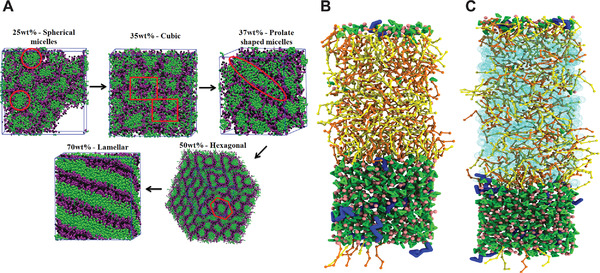
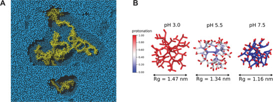
The Martini model, a coarse-grained force field initially developed with biomolecular simulations in mind, has found an increasing number of applications in the field of soft materials science. The model's underlying building block principle does not pose restrictions on its application beyond biomolecular systems. Here, the main applications to date of the Martini model in materials science are highlighted, and a perspective for the future developments in this field is given, particularly in light of recent developments such as the new version of the model, Martini 3.

Keywords: Martini; coarse-graining; molecular dynamics.

Figure 1

Martini mapping examples of selected molecules. A) Standard water particle representing four water molecules; B) the organic solvent toluene; C) dimyristoylphosphatidylcholine (DMPC) lipid; D) poly(ethylene oxide) (PEO); E) the 1‐octyl‐3‐methylimidazolium tetrafluoroborate [C₈mim]⁺[BF₄]⁻ ionic liquid; F) poly(3‐hexylthiophene) (P3HT); G) the 1,3,5‐benzenetricarboxamide (BTA) self‐assembling molecule; H) C₆₀ fullerene; I) the surface of graphene. Martini CG beads are shown as cyan transparent beads overlaying the atomistic structure.

Figure 2

Typical conformations for a chitosan‐based hydrogel with a polymer concentration of 8.9%, and pH of >10.5 (left), 6.5 (middle), and <2.5 (right). Adapted with permission.^{[ 90 ]} Copyright 2017, Royal Society of Chemistry.

Figure 3

Adsorption of polymers and small molecules on surfaces. A) Adsorption of solvated polymer chains on a silica surface. Polymer solvation was found to play a key role for the adsorption of polymers on the silica substrate, highlighting the importance of an explicit description of the solvent in such studies.^{[ 64 ]} B) Self‐assembly on graphite: formation of long‐range ordered lamellar structures of self‐assembling (functionalized) alkanes physisorbed on graphite.^{[ 100 ]} A) Reproduced with permission.^{[ 64 ]} Copyright 2018, American Chemical Society. B) Reproduced with permission.^{[ 100 ]} Copyright 2019, American Chemical Society.

Figure 4

Block copolymer morphologies and self‐assembly. A) Hexagonally packed PDMS cylinders (left‐hand side) and lamellar morphology (right‐hand side). poly(y‐benzyl‐l‐glutamate) (PBLG) is rendered in red, and PDMS in blue.^[54] B) Morphology obtained from the self‐assembly of PEO‐b‐PBMA block copolymers (BCP) in water and THF mixtures. The morphology changes from dissolved chains or monomers in THF, over dispersed sheets or disk‐like aggregates, to vesicles as the fraction of water increases. The morphologies are also affected by the BCP concentration.^{[ 123 ]} A) Reproduced with permission.^{[ 54 ]} Copyright 2014, American Chemical Society. B) Reproduced with permission.^{[ 123 ]} Copyright 2020, Elsevier.

Figure 5

Nanoparticle–polymer systems. Jellyfish‐like and octopus‐like morphology of gold nanoparticles grafted with polymers in a polar and apolar solvent, respectively. Reproduced with permission.^{[ 80 ]} Copyright 2013, Wiley‐VCH.

Figure 6

Simulation of organic electronic materials. A) Bulk heterojunction morphologies from solvent evaporation simulations for a P3HT–PCBM mixture.^{[ 53 ]} The inset shows the resulting atomistic structure obtained via backmapping. P3HT polymer chains are rendered in red and PCBM molecules in blue, respectively. B) Molecular orientations at the donor–acceptor (DA) interface can be resolved, also as a function of molecular features and processing conditions.^{[ 193 ]} A) Reproduced with permission.^{[ 53 ]} Copyright 2017, American Chemical Society. B) Adapted with permission.^{[ 193 ]} Copyright 2020, Wiley‐VCH.

Figure 7

Simulation of morphologies of ion‐conducting materials. A) Representative morphologies of poly(3,4‐ethylenedioxythiophene):polystyrene sulfonate (PEDOT:PSS) systems as a function of the (PSS) deprotonation level, α, which is a function of the pH.^{[ 199 ]} For α = 0 all PSS chains are protonated (PSSH), vice versa for α = 1. The water phase (left‐hand side) is colored in red, blue, or cyan, when the water molecules are within a distance of 6 Å  from PEDOT, PSS, or both, respectively. B) Martini models of anion exchange membranes for fuel cells.^{[ 210 ]} Introduction of 10% of quaternary ammonium (QA) phthalocyanine (Pc) groups (Pc‐PPO‐10) (a) induces a more structured self‐assembly than the random morphology formed by Pc‐PPO‐0 (where QA‐Pc groups are not present) (b), leading to enhanced hydroxide (OH⁻) conductivity. Here, PPO stands for poly(2,6‐dimethyl‐1,4‐phenylene oxide). A) Adapted with permission.^{[ 199 ]} Copyright 2019, Royal Society of Chemistry. B) Adapted with permission.^{[ 210 ]} Copyright 2020, Wiley‐VCH.

Figure 8

Examples of supramolecular polymers. A) Formation of BTA supramolecular polymers, as resolved by Martini CG simulations, proceeds via an initial fast aggregation followed by a slower reorganization and fiber growth.^{[ 257 ]} B) Modeling of porphyrin‐based supramolecular copolymers: the presence of DMAP small‐molecules eases porphyrin monomer exchange in and out the fiber, as quantified by the free energy profiles.^{[ 264 ]} A) Reproduced with permission.^{[ 257 ]} Copyright 2017, American Chemical Society. B) Adapted with permission.^{[ 264 ]} Copyright 2017, American Chemical Society.

Figure 9

Martini modeling of ionic liquids. A) Mesophases formed by the ionic liquid ([C₁₀mim]⁺[BF₄]⁻) water mixtures simulated using Martini for ionic liquids. B,C) Snapshots of the final Martini 3 simulation box of the extraction of polyunsaturated fatty acids from fish oil with an ionic liquid.^{[ 285 ]} In the system (C), octane is added with respect to the composition of system (B), to test the stability of the biphasic system through the addition of co‐solvent. The color coding is as follows: the IL cation representing the imidazolium ring and the alkyl tail is in green, while the IL anion in pink. The polyunsaturated fatty acids to be extracted are in blue, while the palmitic and oleic acids forming the fish oil phase are in yellow and orange, respectively. Octane is depicted in cyan. A) Reproduced with permission.^{[ 284 ]} Copyright 2020, Elsevier. B) Adapted with permission.^{[ 285 ]} Copyright 2020, Royal Society of Chemistry.

Figure 10

Modeling of materials with Martini: recent developments. A) Melt of Martini PS ₁₀₀₀ generated using Polyply.^{[ 65 ]} Highlighted in gold is a single chain with other chains (blue spheres) removed within a cut‐off of 2.3 nm. The total system size is about (30 nm)³. B) Protonation of a poly(propylene imine) (PPI) dendrimer as a function of pH as modeled with the titratable version of Martini.^{[ 303 ]} The protonation state of the core beads of the dendrimer, which represent tertiary amines, clearly changes as a function of pH, becoming progressively less protonated as indicated with the color scale from red (protonated most of the time) to blue (deprotonated most of the time). The radius of gyration (Rg) quantifies the degree of polymer collapse as the charge density decreases at higher pH. B) Reproduced with permission.^{[ 303 ]} Copyright 2020, American Institute of Physics.

References

1. Ingólfsson H. I., López C. A., Uusitalo J. J., de Jong D. H., Gopal S. M., Periole X., Marrink S. J., WIREs Comput. Mol. Sci. 2014, 4, 225. - PMC - PubMed
1. Takada S., Kanada R., Tan C., Terakawa T., Li W., Kenzaki H., Acc. Chem. Res 2015, 48, 3026. - PubMed
1. Joshi S. Y., Deshmukh S. A., Mol. Simul. 2020, 10.1080/08927022.2020.1828583. - DOI
1. Marrink S. J., Risselada H. J., Yefimov S., Tieleman D. P., de Vries A. H., J. Phys. Chem. B 2007, 111, 7812. - PubMed
1. Marrink S. J., de Vries A. H., Mark A. E., J. Phys. Chem. B 2004, 108, 750.
LinkOut - more resources