Integrating barcoded neuroanatomy with spatial transcriptional profiling enables identification of gene correlates of projections

Abstract

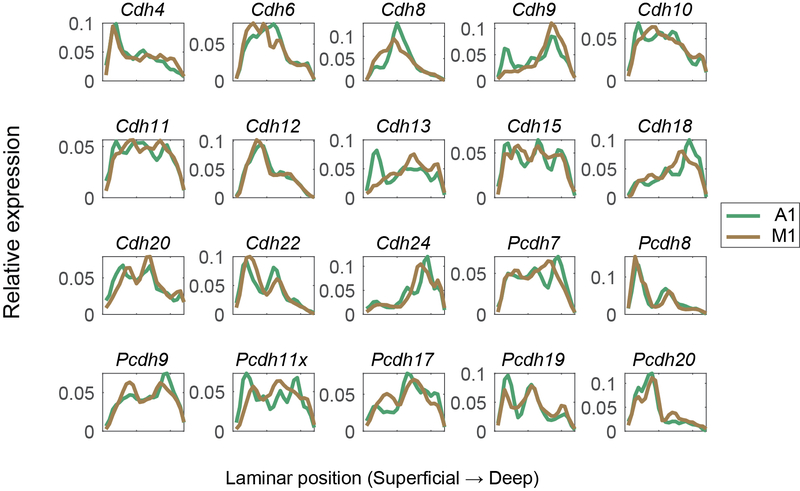
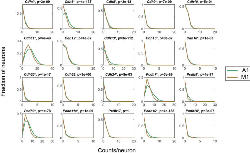
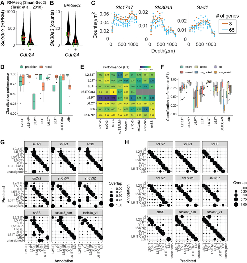
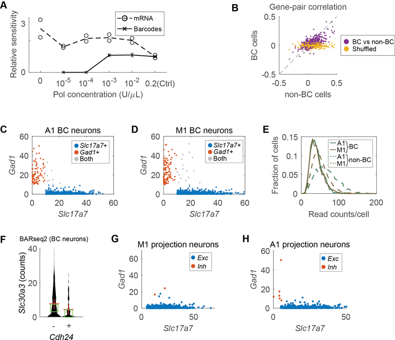
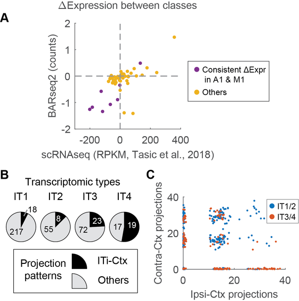
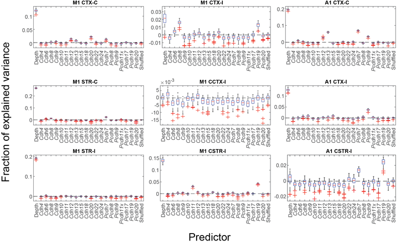
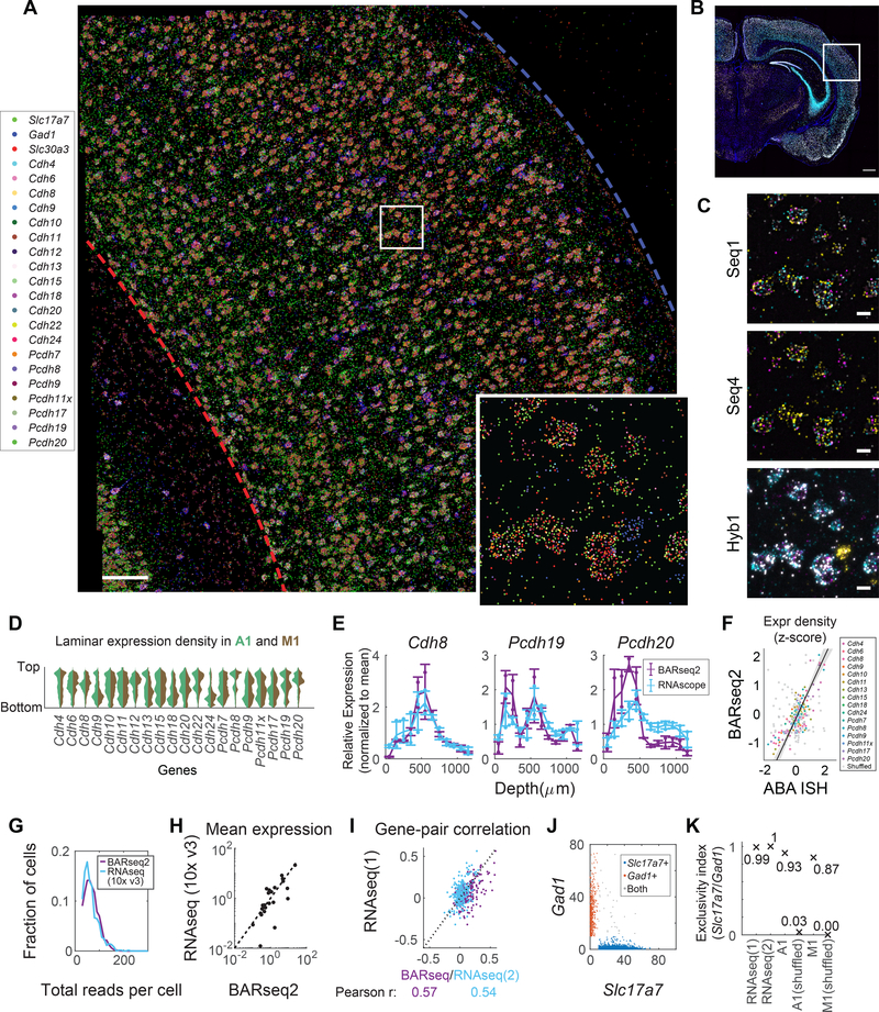
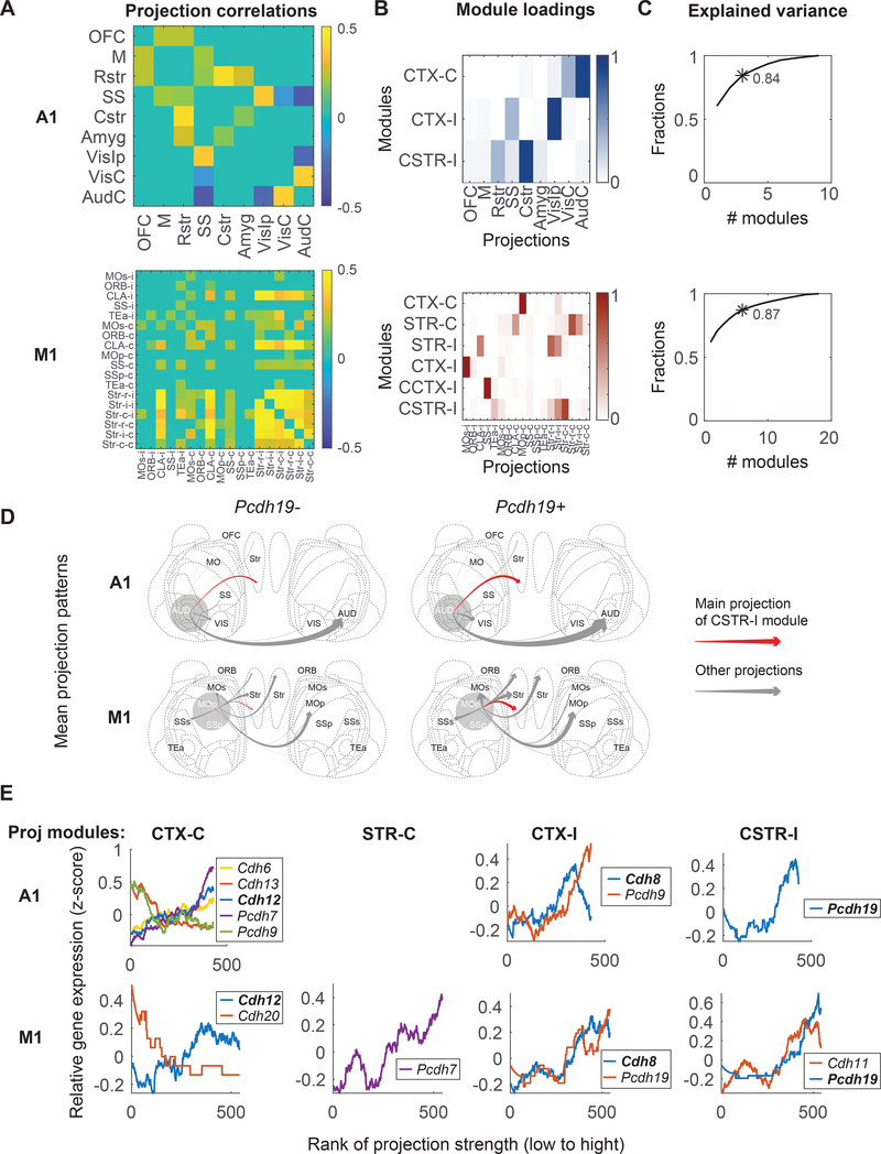
Functional circuits consist of neurons with diverse axonal projections and gene expression. Understanding the molecular signature of projections requires high-throughput interrogation of both gene expression and projections to multiple targets in the same cells at cellular resolution, which is difficult to achieve using current technology. Here, we introduce BARseq2, a technique that simultaneously maps projections and detects multiplexed gene expression by in situ sequencing. We determined the expression of cadherins and cell-type markers in 29,933 cells and the projections of 3,164 cells in both the mouse motor cortex and auditory cortex. Associating gene expression and projections in 1,349 neurons revealed shared cadherin signatures of homologous projections across the two cortical areas. These cadherins were enriched across multiple branches of the transcriptomic taxonomy. By correlating multigene expression and projections to many targets in single neurons with high throughput, BARseq2 provides a potential path to uncovering the molecular logic underlying neuronal circuits.

Extended Data Fig. 1. Optimization of BARseq2 for detecting endogenous mRNAs.

(A) Relative sensitivity (means and individual data points) of BARseq2 in detecting Slc17a7 using the indicated fixation times, normalized to that achieved with 5 mins of fixation. n = 3 for 480 mins and n = 4 for other conditions. (B) Rolony counts for Slc17a7 using either random primers or specific primers at two different concentrations. The two concentrations used were 5 μM (low) and 50 μM (high) for random primers, and 0.5 μM (low) and 5 μM (high) for specific primers. Lines indicate means and dots/crosses represent individual samples. n = 2 slices for each condition. (C) (D) BARseq2 sensitivity compared to RNAscope. (C) Spot density detected by BARseq2 or RNAscope in each 100 μm bin along the laminar axis in auditory cortex. Error bars indicate standard errors. The dashed line indicates linear fit for Slc30a3 and Cdh13. Slope = 1.65 and R² = 0.73. n = 5 slices for both BARseq2 and RNAscope. (D) shows the means and individual samples for each gene. (E)(F) Positions of rolonies across five sequencing cycles using the original (E) or the optimized (F) sequencing protocol. Scale bars = 10 μm. (G) The distribution of minimum distance between rolonies imaged in the first cycle and in the fifth cycle using the original or the optimized protocol. (H) Median distance between rolonies imaged in the indicated cycles and the closest rolonies imaged in the first cycle using the original or the optimized protocol. Error bars indicate standard errors. For both (G) and (H), n = 148,708 rolonies for optimized condition and n = 12,114 for original condition. (I)(J) The distribution of absolute rolony intensities for the first sequencing cycle (I) and relative rolony intensities after 6 sequencing cycles and one stripping step, normalized to the intensities in the first sequencing cycle (J). Amino-allyl dUTP concentrations used are indicated. In (I), n = 63,852 rolonies for 0.08 μM and n = 4,286 rolonies for 0.5 μM; in (J), n = 128,976 rolonies for 0.08 μM and n = 113,235 rolonies for 0.5 μM.

Extended Data Fig. 2. Laminar distribution of cadherins in auditory cortex (green) and motor cortex (brown).

In both cortical areas, cortical depth is normalized so that the bottom and the top of the cortex match between M1 and A1.

Extended Data Fig. 3. Comparison between BARseq2 and Allen gene expression atlas.

Gene expression patterns in auditory cortex identified by BARseq2 are plotted next to in situ hybridization images of the same genes in Allen gene expression atlas (ABA) and the quantified laminar distribution of the gene in both datasets. Only genes that had coronal images in the Allen gene expression atlas are shown. Blue lines indicate the boundaries of the cortex in both BARseq2 and ABA images. In the laminar distribution plots, dots represent values from two BARseq2 samples (purple) and one ABA sample (blue) per gene. Lines indicate means across samples.

Extended Data Fig. 4. The distribution of read counts per cell for the indicated genes in auditory cortex (green) and motor cortex (brown).

Asterisks indicate genes with significant difference in expression between the two areas (p < 0.05 using two-tailed rank sum test after Bonferroni correction). p values after Bonferroni correction are indicated on top.

Extended Data Fig. 5. Transcriptomic typing using BARseq2.

(A)(B) Slc30a3 expression in excitatory neurons with or without Cdh24 expression in single-cell RNAseq (A) from Tasic, et al. or in BARseq2 (B). A cell is considered expressing Cdh24 if the expression is higher than 10 RPKM in RNAseq or 1 count in BARseq2. Red crosses indicate means and green squares indicate medians. (C) Expression density (means and individual data points) across laminar positions for the indicated genes. n = 3 slices for the three-gene panel and n = 5 slices for the 65-gene panel. (D) Precision and recall of cell typing using the marker gene panel across nine single cell datasets. N = 9 independent datasets shown in (E). In each box, the center shows the median, the bounds of the box show the 1^st and 3^rd quartiles, the whiskers show the range of the data, and points further than 1.5 IQR (Inter-Quartile Range) from the box are shown as outliers. (E) Breakdown of average performance for each cell type in each dataset. The datasets are: scSSALM and scSSV1 are single cell SmartSeq datasets from ALM and V1 respectively . All other datasets are BICCN M1 datasets and the name indicates the technology used (sc = single cell, sn = single nuclei, Cv2/3 = Chromium v2/3, SS = SmartSeq). (F) Average cell typing performance for six normalization strategies. N = 9 independent datasets shown in (E). The box plots are generated in the same way as (D). (G) Confusion matrix showing overlap between prediction and annotations, normalized by predictions. This plot emphasizes precision; it indicates the probability that a given prediction was correct. (H) Confusion matrix showing overlap between prediction and annotations, normalized by annotations. This plot emphasizes recall; it indicates the probability that a given annotation was recovered.

Extended Data Fig. 6. Correlating gene expression to projections using BARseq2.

(A) Relative sensitivity of BARseq2 to barcodes (solid line) and endogenous mRNAs (dashed line) using the indicated concentration of Phusion DNA polymerase. Sensitivities are normalized to the original BARseq condition (Ctrl). Circles and crosses show individual data points across n = 2 slices. (B) Correlation between pairs of genes in barcoded cells (y-axis) and in non-barcoded cells (x-axis) as determined by BARseq2. Shuffled data (yellow) are also plotted for comparison. (C)(D) Slc17a7 (x-axes) and Gad1 (y-axes) expression in barcoded neurons in auditory (C) or motor cortex (D). Only neurons with more than 10 counts in either gene are shown. (E) The distributions of read counts per barcoded neuron (solid lines) or non-barcoded neuron (dashed lines) in auditory (green) and motor (brown) cortex. (F) Slc30a3 expression in barcoded excitatory neurons with or without Cdh24 expression in BARseq2. A cell is considered expressing Cdh24 if the expression is higher than 1 count. Red crosses indicate means and green squares indicate median. (G)(H) Slc17a7 (x-axes) and Gad1 (y-axes) expression in barcoded projection neurons in motor (G) or auditory cortex (H). Excitatory and inhibitory neurons are color-coded as indicated.

Extended Data Fig. 7. BARseq2 reveals projection and gene expression differences across major classes and IT subtypes.

(A) Differential gene expression across major classes (IT, PT, and CT) observed using BARseq2 and single-cell RNAseq. Each dot shows the difference in mean expression of a gene across a pair of major classes observed using BARseq2 (y-axis) or single-cell RNAseq (x-axis). Differences in expression that were statistically significant (FDR < 0.05 using two-tailed rank sum tests) in both A1 and M1 as shown by BARseq2 are labeled purple; otherwise they are labeled yellow. The single-cell RNAseq data used were collected in the visual cortex and anterior-lateral motor cortex . (B) The fraction of ITi-Ctx neurons in four transcriptomic types of IT neurons in auditory cortex. ITi-Ctx neurons have only ipsilateral cortical projections and no striatal projections or contralateral projections . The number of ITi-Ctx neurons and neurons with other projection patterns for each transcriptomic type are labeled on top of the pie charts. (C) The projection strengths for contralateral (y-axis) and ipsilateral (x-axis) cortical projections for each IT neuron in auditory cortex. IT1/IT2 neurons are labeled blue and IT3/IT4 neurons are labeled red.

Extended Data Fig. 8. Variance in projections explained by cadherins and laminar positions.

Box plots of variance in each projection modules explained by the indicated predictors after 100 iterations of 10-fold cross validation. Boxes indicate second and third quartiles and whiskers indicate minimum and maximum values excluding outliers. Outliers are shown in red.

Extended Data Fig. 9. Validation of correlation between cadherins and IT projections.

(A) Representative images of in situ hybridization in A1 (top) and M1 (bottom) slices with CTB labeling in the caudal striatum. Three marker genes and CTB labeling are shown in the indicated colors. Scale bars = 100 μm. Arrows and arrowheads indicate example CTB+ and CTB- neurons, respectively. Experiments for each combination of targeted gene and CTB labeling condition (Cdh12 with contralateral labeling, Cdh8 with ipsilateral labeling, and Pcdh19 with striatal labeling) were performed in slices from two animals. (B) Crops of the indicated individual channels of example neurons from (A). Scale bars = 10 μm. (C)(D)(E) Cumulative probability distribution of the expression of Cdh12 (C), Cdh8 (D), and Pcdh19 (E) in neurons with or without retrograde labeling of contralateral (C), ipsilateral (D), or caudal striatal (E) projections. p values from two-tailed rank sum tests after Bonferroni correction and numbers of neurons used for each experiment are indicated. N = 2 animals for each experiment.

Extended Data Fig. 10. Cadherin co-expression modules correlate with IT projections.

(A) Correlation among cadherins in IT neurons in motor cortex identified in the indicated single-cell RNAseq datasets ^,. The datasets included are: tasic_alm and tasic_v1 are single cell SmartSeq datasets from ALM and V1 respectively ; all other datasets are BICCN M1 datasets ; the name indicates the technology used (sc = single cell, sn = single nuclei, Cv2/3 = Chromium v2/3, SS = SmartSeq). (B) Modularity (EGAD AUROC) of co-expression modules in BARseq2 M1 against null distribution of modularity (node permutation). BARseq2 modularity is shown by the blue lines with the corresponding p-values. P values are calculated using a one-sided non-parametric node permutation test without multiple comparison correction. (C) Association (AUROC) between cadherin co-expression modules and the indicated projections. Significant associations are marked by asterisks (* FDR < 0.1, ** FDR < 0.05). (D) Fractions of neurons with the indicated projections as a function of co-expression module expression. (E) Distribution of associations of the indicated projection modules with gene expression. Association with significant gene module is shown by a blue line; association with single genes from that module is shown by orange lines; association with all other genes is shown by a gray density. (F) Association of the three co-expression modules in transcriptomic IT neurons in the indicated datasets (AUROC, significance shown as in C).

Figure 1.. In situ sequencing of endogenous mRNAs using BARseq2.

(A) Cartoon of an example model in which the relationship between projections and gene expression can only be correctly inferred by multiplexed interrogation of both projections and gene expression. In this model (Top), neurons that express both genes project to both targets A and B, whereas neurons that express only one of the two genes project randomly to either A or B, but not both. (Bottom left) Methods that combine multiplexed single neuron gene expression with data about only a single projection target will conclude that all three gene expression patterns project to target A, and thus fail to detect the underlying “true” relationship between gene expression and projections. (Bottom right) Similarly, methods that combine multiplexed single neuron projections with data about only a single gene will also fail to detect any relationship between gene expression and projections. (B)(C) BARseq2 correlates projections and gene expression at cellular resolution. In BARseq2, neurons are barcoded with random RNA sequences to allow projection mapping, and genes are also sequenced in the same barcoded neurons. RNA barcodes and genes are amplified and read out using different strategies (C). (D) Theoretical imaging cycles using combinatorial coding (BARseq2), 4-channel sequential coding, or 4-channel sparse coding as used by Eng, et al. . Imaging cycles assumed 3 additional cycles for BARseq2, 1 additional round for sparse coding, and no extra cycle for sequential coding for error correction. (E) Mean and individual data points of the relative sensitivity of BARseq2 in detecting the indicated genes using different numbers of padlock probes per gene. The sensitivity is normalized to that using one probe per gene. n = 2 slices for each gene. (F) Representative images of BARseq2 (bottom) detection of the indicated genes using the maximum number of probes shown in (E) compared to RNAscope (top). Scale bars = 10 μm.

Figure 2.. Multiplexed detection of mRNAs using BARseq2.

(A) A representative image of rolonies in auditory cortex (out of two slices sequenced). Scale bar = 100 μm. The inset shows a magnified view of the boxed area. (B) Low magnification image of the hybridization cycle showing the location of the area imaged in A. Scale bar = 100 μm (C) Representative images of the indicated sequencing cycle and hybridization cycle of the boxed area in A. Scale bars = 10 μm. (D) Violin plots showing the laminar distribution of cadherin expression in neuronal somata. Expression in auditory cortex and motor cortex is shown in different colors as indicated. (E) Laminar distribution of gene expression as detected by BARseq2 or FISH. Lines indicate means, error bars indicate standard deviations, and dots show individual data points. n = 2 slices for BARseq2 and n = 3 slices for FISH. (F) Relative gene expression observed using BARseq2 and in Allen gene expression atlas. Each dot represents the expression of a gene in a 100 μm bin in laminar depth. Gray dots indicate correlation between data randomized across laminar positions. A linear fit and 95 % confidence intervals are shown by the diagonal line and the shaded area. n = 2 slices for BARseq2 and n = 1 slice for ABA ISH. (G) Distribution of total read counts per cell in BARseq2 and single-cell RNAseq in auditory cortex. Only genes used in the panel detected by BARseq2 were included. (H) Mean expression for each gene detected using BARseq2 or single-cell RNAseq. Each dot represents a gene. The dotted line indicates equal expression between BARseq2 and single-cell RNAseq. (I) The correlation between pairs of genes observed in BARseq2 and single-cell RNAseq (purple dots), or in two single-cell RNAseq datasets (blue dots). (J) Expression of Slc17a7 and Gad1 in single neurons. Color codes indicate whether the neuron dominantly expressed Slc17a7 (blue) or Gad1 (red), or expressed both strongly (gray). (K) Exclusivity indices (see Methods) of Slc17a7 and Gad1 in neurons in two single-cell RNAseq datasets, BARseq2 in auditory or motor cortex, and shuffled BARseq2 data.

Figure 3.. Cadherin expression across transcriptomic neuronal types in motor cortex.

(A) A representative image of rolonies in motor cortex (out of four slices sequenced). mRNA identities are color-coded as indicated. The top and the bottom of the cortex are indicated by the blue and red dashed lines, respectively. Scale bar = 100 μm. (B) Transcriptomic cell types called based on gene expression shown in (A). (C) Laminar distribution of transcriptomic neuronal types based on marker gene expression observed by BARseq2. Layer identities are shown on the right. (D) Differential expression of cadherins across transcriptomic neuronal types identified by BARseq2. Over-expression is indicated in yellow and under-expression is indicated in blue. Only differential expression that was statistically significant was shown. Statistical significance was determined using two-tailed rank sum test with Bonferroni correction for each gene between the indicated transcriptomic type and the expression of that gene across all other neuronal types.

Figure 4.. Correlating gene expression to projections using BARseq2.

(A) False-colored barcode sequencing images (left), soma segmentations (middle), and gene rolonies (right) of three representative neurons from the motor cortex. The segmentation and gene rolony images correspond to the white squared area in the barcode images. In the gene rolony images, the areas corresponding to the soma segmentations of the target neurons are in black. All scale bars = 20 μm. (B) Projections (left) and gene expression (right) of the target neurons shown in (A). The dots indicating gene expression are colored using the same color code as that in the gene rolony plots in (A). The neurons shown in the first two rows are excitatory projection neurons, whereas the neuron shown in the bottom row is an inhibitory neuron without projections. See Supp. Table S2 for the brain areas corresponding to each abbreviated target area. (C) Projections (left) and gene expression (right) of neurons in auditory cortex (top) and motor cortex (bottom). Each row represents a barcoded projection neuron. Both projections and gene expression are shown in log scale. Major projection neuron classes determined by projection patterns are indicated on the right. (D) (E) The number of excitatory neurons (blue) or inhibitory neurons (red) in all barcoded neurons (D) or barcoded projection neurons (E). Neurons in auditory cortex are shown in the top row and those in motor cortex are shown in the bottom row.

Figure 5.. Differential cadherin expression across major classes and cortical areas.

(A) Vertical histograms of the expression (raw counts per cell) of cadherins that were differentially expressed across major classes in either auditory or motor cortex. Y-axes indicate gene expression level (counts per cell) and x-axes indicate number of neurons at that expression level. The numbers of neurons are normalized across plots so that the bins with the maximum number of neurons have equal bar lengths. Gene expression in auditory cortex (green) are shown on the left in each plot, and gene expression in motor cortex (brown) are shown on the right in each plot. Lines beneath each plot indicate pairs of major classes with different expression of the gene (FDR < 0.05). (B)(C) Volcano plots of cadherins that were differentially expressed across pairs of major classes in auditory cortex (B) or motor cortex (C). Y-axes indicate significance and x-axes indicate effect size. The horizontal dashed lines indicate significance level for FDR < 0.05, and the vertical dashed lines indicate equal expression. (D) Volcano plots of cadherins that were differentially expressed across auditory and motor cortex in the indicated major classes. Y-axes indicate significance and x-axes indicate effect size. The horizontal dashed lines indicate significance level for FDR < 0.05, and the vertical dashed lines indicate equal expression. For all panels, p values are calculated using two-tailed rank sum tests.

Figure 6.. Cadherins correlate with diverse projections of IT neurons.

(A) Pearson correlation of projections to different brain areas in IT neurons of auditory cortex (top) or motor cortex (bottom). Only significant correlations are shown. (B) Projection modules of IT neurons in auditory cortex (top) or motor cortex (bottom). Each row represents a projection module. Columns indicate projections to different brain areas. (C) The fractions of variance explained by different numbers of projection modules in auditory cortex (top) and motor cortex (bottom). The numbers of projection modules that correspond to those in (B) are labeled with an asterisk with the fraction of variance explained indicated. (D) Mean projection patterns of neurons in A1 (top) and M1 (bottom) with or without Pcdh19 expression. The thickness of arrows indicates projection strength (barcode counts). Red arrows indicate projections that correspond to the strongest projection in the CSTR-I projection modules. (E) The expression of cadherins (y-axes) that were rank correlated with the indicated projection modules in auditory cortex (top row) and motor cortex (bottom row). Neurons (x-axes) are sorted by the strengths of the indicated projection modules. Only genes that were significantly correlated with projection modules are shown (FDR < 0.1 using two-tailed rank sum tests). Genes that were correlated with the same projection modules in both areas are shown in bold.

Figure 7.. Gene co-expression modules correlate with diverse projections of IT neurons.

(A) Correlation among cadherins as identified using single-cell RNAseq in IT neurons in motor cortex . Three co-expression modules are marked by red squares. Cadherins that did not belong to any module were not shown. (B) Association between cadherin co-expression modules and projection modules (AUROC). Significant associations are marked by asterisks (*FDR < 0.1, **FDR < 0.05). (C) Fractions of neurons with the indicated projection modules as a function of co-expression module expression. Neurons are binned by gene module quantiles as indicated. (D) Association of the three co-expression modules in transcriptomic IT neurons in the scSS dataset (AUROC, significance shown as in B).

References

1. Winnubst J et al. Reconstruction of 1,000 Projection Neurons Reveals New Cell Types and Organization of Long-Range Connectivity in the Mouse Brain. Cell 179, 268–281 e213, doi:10.1016/j.cell.2019.07.042 (2019). - DOI - PMC - PubMed
1. Muñoz-Castañeda R et al. Cellular Anatomy of the Mouse Primary Motor Cortex. bioRxiv, 2020.10.02.323154, doi:10.1101/2020.10.02.323154 (2020). - DOI - PMC - PubMed
1. Tasic B et al. Shared and distinct transcriptomic cell types across neocortical areas. Nature 563, 72–78, doi:10.1038/s41586-018-0654-5 (2018). - DOI - PMC - PubMed
1. Zeisel A et al. Molecular Architecture of the Mouse Nervous System. Cell 174, 999–1014 e1022, doi:10.1016/j.cell.2018.06.021 (2018). - DOI - PMC - PubMed
1. Han Y et al. The logic of single-cell projections from visual cortex. Nature 556, 51–56, doi:10.1038/nature26159 (2018). - DOI - PMC - PubMed
Method References
1. Oh SW et al. A mesoscale connectome of the mouse brain. Nature 508, 207–214, doi:10.1038/nature13186 (2014). - DOI - PMC - PubMed
1. Edelstein AD et al. Advanced methods of microscope control using μManager software. J Biol Methods 1, e10, doi:10.14440/jbm.2014.36 (2014). - DOI - PMC - PubMed
1. Lee JH et al. Highly multiplexed subcellular RNA sequencing in situ. Science 343, 1360–1363, doi:10.1126/science.1250212 (2014). - DOI - PMC - PubMed
1. Evangelidis GD & Psarakis EZ Parametric image alignment using enhanced correlation coefficient maximization. IEEE Trans Pattern Anal Mach Intell 30, 1858–1865, doi:10.1109/TPAMI.2008.113 (2008). - DOI - PubMed
1. Stringer C, Wang T, Michaelos M & Pachitariu M Cellpose: a generalist algorithm for cellular segmentation. bioRxiv, 2020.02.02.931238, doi:10.1101/2020.02.02.931238 (2020). - DOI - PubMed
Publication types