Neural network aided approximation and parameter inference of non-Markovian models of gene expression

Abstract

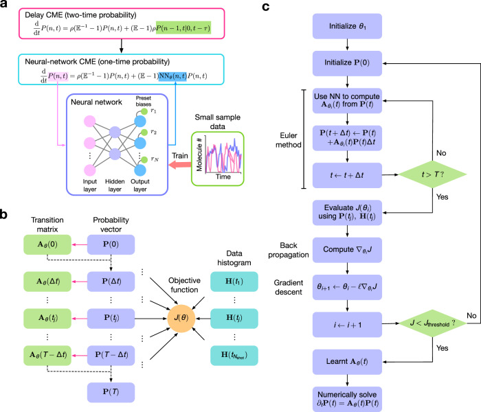
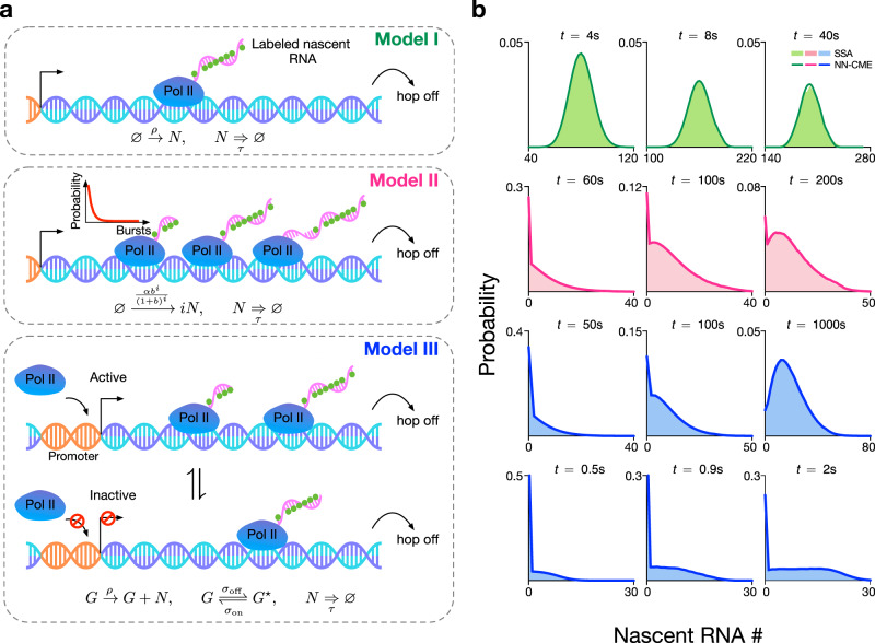
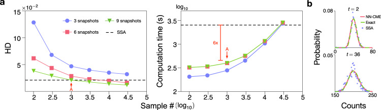
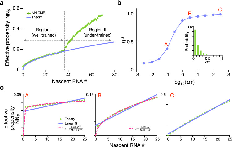
Non-Markovian models of stochastic biochemical kinetics often incorporate explicit time delays to effectively model large numbers of intermediate biochemical processes. Analysis and simulation of these models, as well as the inference of their parameters from data, are fraught with difficulties because the dynamics depends on the system's history. Here we use an artificial neural network to approximate the time-dependent distributions of non-Markovian models by the solutions of much simpler time-inhomogeneous Markovian models; the approximation does not increase the dimensionality of the model and simultaneously leads to inference of the kinetic parameters. The training of the neural network uses a relatively small set of noisy measurements generated by experimental data or stochastic simulations of the non-Markovian model. We show using a variety of models, where the delays stem from transcriptional processes and feedback control, that the Markovian models learnt by the neural network accurately reflect the stochastic dynamics across parameter space.

Fig. 1. The ANN-aided stochastic model approximation.

a Illustration of the key idea behind the method, namely the ANN-aided mapping of a delay master equation that is in terms of the two-time probability distribution by the simpler neural-network chemical master equation (NN-CME) whose terms are only a function of the current time. b Illustration of the procedure behind the calculation of the transition matrix and the objective function. For a given set of weights and biases of the ANN (denoted by θ), taking as input P(t), the ANN’s output gives the transition matrix elements A_θ(t), which then by means of the Euler method (or more advanced differential equation solvers) is used to predict the distribution at the next time step P(t + Δt). Note that magenta arrows show the ANN computation while the black dashed arrows show the use of the Euler method. Stochastic simulations that sample the solution of the delay master equation are used to produce histograms at several time points H(t); finally the distance J(θ) is calculated between the latter and P(t) (evaluated at the same time points). c Flowchart illustrating all the steps in ANN training. If the objective function calculated as shown in (b) is above a threshold then the weights and biases of the ANN are updated using back propagation followed by gradient descent; this is repeated until the objective function is below a threshold.

Fig. 2. ANN-aided stochastic model approximation of various models of transcription.

a Illustration of three models of transcription. The models describe initiation, elongation and termination and specifically predict the numbers of nascent RNAs (equivalently the number of RNAP polymerases, Pol IIs) at the gene locus. In all models, a nascent RNA molecule detaches after a constant time has elapsed from its binding to the promoter. The models differ in how they model Pol II binding: in Model I, the binding is modelled as a Poisson process, hence one at a time; in Model II, binding occurs in bursts, whose size conforms to a geometric distribution; in Model III, the gene switches between active and inactive states, and only the active state permits Pol II binding. b For all models, the FSP solution of the NN-CME derived by the ANN-aided procedure is in excellent agreement with the SSA of the delay CME. The accuracy is independent of the modality and skewness of the distribution. The rate constants and other parameters related to the ANN’s training are specified in SI Table 1.

Fig. 3. Evaluating the performance of the ANN-aided model approximation.

a Precision and computational efficiency of the ANN-aided model approximation as a function of sample size and number of snapshots. The method is benchmarked on Model I since the time-dependent solution of the delay CME is exactly known (see SI Note 1) and hence the accuracy of our method can be precisely quantified. A measure of the accuracy is the average Hellinger distance (HD) between the NN-CME and exact distributions at four different time points. The computation time is equal to the time-to-acquire samples plus time for training. Each data point in the graphs is averaged on three independent trainings. Note that the NN-CME obtained from training with 10³ samples produces a distribution that is as precise as that from 3 × 10⁴ samples using the SSA of the delay CME (shown as a black dashed line); in this case the computation time of the NN-CME is also just 1/6 of the SSA. b Comparison of the NN-CME distributions, exact analytical distributions and histograms from stochastic SSA simulations of the delay CME at two different time points; the sampling for both training and the SSA is 10³. Note that the NN-CME leads to much more accurate distributions than the SSA for the same number of samples. The rate constants and other parameters related to the ANN’s training are specified in SI Table 1.

Fig. 4. Effective degradation propensity of Model II.

a Comparison of the effective degradation propensity NN_θ(n) in steady-state conditions predicted by theory (solid purple line; Eq. S36 in the SI) and computed by the ANN-aided approximation (green dots). Note that the two agree in Region I where the nascent RNA probability is sufficiently high so that the neural-network coefficients are well-trained. The two are not matched in Region II, since the neural-network coefficients are under trained such that the neural-network output is not reliable. b Shows the square of the Pearson correlation coefficient R² between the effective propensity and the nascent RNA number as a function of the non-dimensional parameter ατ. The non-linearity of the effective propensity rapidly increases as the burst frequency α decreases below the elongation frequency τ⁻¹. Inset shows the histogram of ατ for 368 genes in mouse embryonic stem cells (see SI Note 6 for details of the histogram). c Shows the effective propensity as a function of nascent RNA numbers for points A, B and C labelled in (b). The function is almost independent of nascent RNA number for small ατ (point A), well-approximated by a Hill function of the nascent RNA number for intermediate ατ (point B), and a linear function of nascent RNA number for large ατ (point C). Note that the Hill function fits (for points A and B) are only valid over the region shown and break down for larger n. The kinetic parameters of Model II are the same as Fig. 2 and the NN-CME is trained at steady state (solving A_θ(t)P(t) = 0) using 2 × 10⁵ samples.

Fig. 5. Stochastic bifurcation diagram for Model III in the bursty regime (σ_off ≫ σ_on) using the NN-CME and comparison with theory.

a From an analytical approximation of Model III in the bursty regime, the space is divided into four regions according to the type of distributions (shown in b): type I, a unimodal distribution with mode = 1; type II, a unimodal distribution with mode = 0; type III, a unimodal distribution with mode > 1; type IV, a bimodal distribution with two modes at zero and a non-zero value. Region IV is highlighted in green since it is a phase that does not exist in the bursty regime of the standard model of gene expression (Model III with delayed degradation replaced by first-order degradation)—this is hence delay-induced bimodality. The lines defining the division of space are: solid line is $\left(2+\frac{2}{b}\right)/\alpha$ and the dashed line is $\left(b+\frac{1}{b}+2\right)/\alpha$, which respectively are the lower and upper bounds on τ given by Eq. (9). To check the accuracy of the ANN-aided model approximation for Model III, we used it to compute the NN-CME and then solved using FSP to obtain nascent number distributions for 200 points in parameter space. These are randomly sampled from the space {ρ = 2.11, σ_off ∈ 2.11 × [10⁻¹, 10], σ_on = 0.0282, τ ∈ [10, 10³]} (left) and {ρ = 2.11, σ_off = 0.609, σ_on = 0.0282 × [10⁻¹, 10], τ ∈ [10, 10³]} (right). Dots denote parameter sets for which the NN-CME distributions are unimodal and crosses show those for which the distributions are bimodal. The fact that the vast majority of crosses fall in region IV and the dots outside of it shows that the NN-CME agrees with the analytical approximation of Model III (parameter sets, which mismatch between the NN-CME and theory, are highlighted with red arrows and are very few in number). Note in the left figure of (a), the burst frequency is fixed to α = 0.0282 (left) while in the right figure, we use α₀ = 0.0282 and the burst size is fixed to b = 3.46. c The NN-CME is learnt from stochastic simulations of the delay model of Model III with the added feature that the elongation time τ is a random variable sampled from two different lognormal distributions (see top figure). In the middle and bottom figures, we show that the delay-induced bimodality (phase IV) disappears as the variance on the elongation time τ increases at constant mean. The rate constants and other parameters related to the ANN’s training are specified in SI Table 1.

Fig. 6. NN-CME accurately predicts the properties of a stochastic auto-regulatory model of oscillatory gene expression when only partial data are used for ANN training.

a Illustration of a model of auto-regulation whereby a protein X is transcribed by a gene, then it is transformed after a delay time τ into a mature protein Y, which binds the promoter and represses transcription of X. The functions J₁(Y) and J₂(Y) can be found in SI Note 7. b Two typical SSA simulations of proteins X and Y, clearly showing that single-cell oscillations while noisy, they are sustained. c, d The NN-CME is obtained from training the ANN using only protein Y data from SSA simulations of the delay model of the auto-regulatory model. Surprisingly, the NN-CME’s solution for the temporal variation of the mean number of both proteins X and Y, and for their distributions is in excellent agreement with that of the SSA. Note the distributions in (d) are for the three time points labelled A, B and C in (c). The rate constants and other parameters related to the ANN’s training are specified in SI Table 1.

Fig. 7. ANN-aided model approximation seamlessly integrates the inference of kinetic parameters and approximation of the delay CME by a NN-CME.

The unknown kinetic parameters can be treated in the same way as neural-network coefficients (weight and biases) and optimized to minimize the objective function. Application to Model II. a Sketch of the computation of the 95% confidence interval (CI) of the inferred kinetic parameters. Blue areas indicate the 95% confidence region, while the grey area shows the non-confidence region. Both solid and dashed red lines show the profile likelihoods (PLs) of burst frequency α and burst size b, respectively (See SI Note 8 for details). b Inferred values of α and burst size b (dots), their 95% CIs (error bars) and the true values (green lines) for five mammalian genes. Inference by using ANN-aided model approximation is robust against size of dataset: Dataset A (blue, 100 snapshots and 10⁴ cells) and Dataset B (red, 50 snapshots and 10³ cells) produce similar results. c Quantile–quantile plots for the steady-state distributions of the NN-CME and those obtained from the SSA; the linearity confirms that the ANN-aided model approximation can accurately approximate the distribution using the NN-CME even when the optimization is over both the kinetic parameters and the neural-network coefficients. The rate constants and other parameters related to the ANN’s training are specified in SI Table 1.

References

1. Shahrezaei V, Swain PS. Analytical distributions for stochastic gene expression. Proc. Natl Acad. Sci. U.S.A. 2008;105:17256–17261. doi: 10.1073/pnas.0803850105. - DOI - PMC - PubMed
1. Cao Z, Grima R. Analytical distributions for detailed models of stochastic gene expression in eukaryotic cells. Proc. Natl Acad. Sci. U.S.A. 2020;117:4682–4692. doi: 10.1073/pnas.1910888117. - DOI - PMC - PubMed
1. Cao Z, Grima R. Linear mapping approximation of gene regulatory networks with stochastic dynamics. Nat. Commun. 2018;9:1–15. doi: 10.1038/s41467-017-02088-w. - DOI - PMC - PubMed
1. Peccoud J, Ycart B. Markovian modeling of gene-product synthesis. Theor. Popul. Biol. 1995;48:222–234. doi: 10.1006/tpbi.1995.1027. - DOI
1. Raj A, Peskin CS, Tranchina D, Vargas DY, Tyagi S. Stochastic mRNA synthesis in mammalian cells. PLoS Biol. 2006;4:e309. doi: 10.1371/journal.pbio.0040309. - DOI - PMC - PubMed
Publication types
LinkOut - more resources